
1. Introduction
The emergence of previously unidentified infectious diseases and pathogens has stimulated much concern in the public health community. This has triggered an interest in the collection of pathogen-specific and epidemiological data to inform risk assessment, management, and mitigation practices. This can be a difficult task given the number of key variables that impact pathogen spread, persistence, transmission, success, and other factors, including changes in the demographics of exposed populations and immunocompetency. For example, pathogen emergence and reemergence in specific geographic locales encompasses everything from previously unidentified infectious agents entering the human population to established pathogens invading new populations and the evolution of drug resistance ( Metcalf and Lessler 2017 [HY5RFF5T] Metcalf, C. Jessica E., and Justin Lessler. 2017. “Opportunities and Challenges in Modeling Emerging Infectious Diseases.” Science 357 (6347): 149–52. https://doi.org/10.1126/science.aam8335. ).
Traditional infectious diseases, together with emerging and reemerging infections, remain a major public health threat globally, and especially in low- and middle-income countries where resources are limited ( Chen et al. 2023 [J57FVEVW] Chen, Wangxue, Francisco García-del Portillo, and Amin Talebi Bezmin Abadi. 2023. “Editorial: Special Issue: Advances in Microbial Pathogenesis.” Microbial Pathogenesis 174 (January): 105926. https://doi.org/10.1016/j.micpath.2022.105926. ). Rapid urbanization, home insecurity, and deteriorating or already poor infrastructure has been changing the pattern of disease outbreaks, morbidity, and mortality. Land-use changes, such as agricultural expansion and deforestation, have changed the transmission of infectious disease directly through changing human contact with wildlife and vectors, but also indirectly through changes in biodiversity and pathogen spread due to increased travel, trade, and globalization. These changes may not only contribute to an increase in the transmission speed of outbreaks but also enlarge the scope of the transmission area ( Wu et al. 2014 [NQAZNGYD] Wu, XiaoXu, HuaiYu Tian, Sen Zhou, LiFan Chen, and Bing Xu. 2014. “Impact of Global Change on Transmission of Human Infectious Diseases.” Science China Earth Sciences 57 (2): 189–203. https://doi.org/10.1007/s11430-013-4635-0. ).
In addition, the significant rise in antimicrobial resistance has compounded the challenge of infectious disease transmission prevention globally ( WHO 2021 [6XKSE37F] WHO. 2021. “Antimicrobial Resistance.” https://www.who.int/news-room/fact-sheets/detail/antimicrobial-resistance. . It was estimated that 1.27 million people died directly from antibiotic-resistant bacterial infections in 2019, and 4.95 million people died from illnesses in which bacterial antimicrobial resistance was implicated ( Murray et al. 2022 [RMMRBBSK] Murray, Christopher J. L., Kevin Shunji Ikuta, Fablina Sharara, et al. 2022. “Global Burden of Bacterial Antimicrobial Resistance in 2019: A Systematic Analysis.” The Lancet 399 (10325): 629–55. https://doi.org/10.1016/S0140-6736(21)02724-0. ). Changes in water and solids recycling can also impact exposure to pathogens. Adoption of direct and indirect potable reuse has several benefits as drought-proof sources of drinking water, particularly in arid regions; however, there are concerns of increased exposure to biological contaminants of emerging concern (BioCEC) such as antibiotic-resistant bacteria and opportunistic pathogens ( Garner et al. 2018 [FICVU29L] Garner, Emily, Chaoqi Chen, Kang Xia, et al. 2018. “Metagenomic Characterization of Antibiotic Resistance Genes in Full-Scale Reclaimed Water Distribution Systems and Corresponding Potable Systems.” Environmental Science & Technology 52 (11): 6113–25. https://doi.org/10.1021/acs.est.7b05419. ).
Climatic hazards, such as sea-level rise, heatwaves, droughts, wildfires, floods, etc., can also impact disease transmission. Mora et al.( Mora et al. 2022 [YAEUUSEC] Mora, Camilo, Tristan McKenzie, Isabella M. Gaw, et al. 2022. “Over Half of Known Human Pathogenic Diseases Can Be Aggravated by Climate Change.” Nature Climate Change 12 (9): 869–75. https://doi.org/10.1038/s41558-022-01426-1. ) reported that out of 375 infectious diseases documented globally, 58% will be aggravated by climatic hazards. The study also reported specific pathways through which climate change aggravation can occur:
- Climatic hazards bringing pathogens closer to people (e.g., increases in vector and pathogen spread, spillover from viruses with viruses moving over larger areas following climatic hazard, storms causing wastewater overflows)
- Climatic hazards bringing people closer to pathogens (e.g., water reclamation and reuse, increased recreational activities during heat waves)
- Climatic hazards increasing the virulence of pathogens (e.g., increases in harmful algal blooms, rainfall increasing habitats for vector-borne disease transmission, heatwaves selecting for “heat-resistant” microorganisms)
- People impaired by climatic hazards (e.g., stress and malnutrition that reduce immunity, people forced into unsafe conditions, damaged infrastructure)
Identifying key variables that predict the increased potential of environmental transmission of pathogens is crucial to proactively take measures to minimize the spread of BioCEC. The objective of this section is to characterize key variables that may be used to identify, evaluate, and prioritize BioCEC. In addition, resources that can be used for prioritization of BioCEC is summarized to help assess the risk of BioCEC and inform decisions. The section does not include person-to-person transmission and community spread of disease, since communicable diseases are not within the scope of this guidance.
Figure 1 shows the framework adapted the Centers for Disease Control and Prevention’s (CDC’s) One Health approach ( CDC 2024 [Q9KEGHPZ] CDC. 2024. “About One Health.” One Health, November 21. https://www.cdc.gov/one-health/about/index.html. ), which illustrates a variety of macro-level factors, including the epidemiological triangle, that influence pathogen or BioCEC transmission and infectious disease risk. The epidemiological triangle (pathogen/BioCEC, host, and environment) in the center of the graphic is the framework used for the discussion of key variables in this section (see The Epidemiological Triangle).
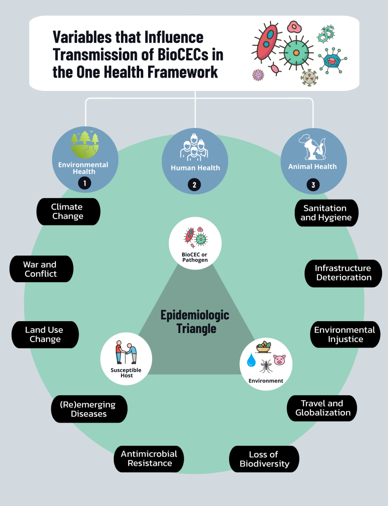
Figure 1. Variables that influence the transmission of biological contaminants of emerging concern in the One Health framework.
Source: Adapted from (
CDC 2024 [Q9KEGHPZ] CDC. 2024. “About One Health.” One Health, November 21. https://www.cdc.gov/one-health/about/index.html.
).
The section is divided into six subsections. The Epidemiological Triangle describes the epidemiological triangle, which is the framework used for the discussion of key variables. This concept is used to describe the relationships and interactions among pathogen, host, and exposure through the environment to determine the impact of BioCEC on human health. These relationships and interactions for a specific BioCEC scenario, outbreak, or site of concern are better illustrated and defined using a site-specific conceptual exposure model (CEM). As defined in the Conceptual Exposure Model, a CEM is a visual representation of a site, such as illustrations or block diagrams, that maps known and potential interactions among an environment, pathogen, and host. The relationships and interactions presented in the CEM inform the identification and evaluation of key variables that influence the presence and severity of a BioCEC scenario or outbreak. Likewise, the evaluation of key variables using newly available information provides feedback for changing the CEM. CEM development and examples are presented in the Conceptual Exposure Model.
In Considerations for Assessing Risks from BioCEC, we define and discuss key variables of each leg of the epidemiologic triangle. Key variables that fall under pathogen, host, and environment are identified and described to provide context for evaluation of risk of BioCEC.
In Approaches to BioCEC Prioritization Strategies, different prioritization schemes that are used to evaluate the risk of BioCEC are reviewed, including the World Health Organization’s (WHO’s) guideline, the US Environmental Protection Agency’s (USEPA’s) Contaminant Candidate List 5 (CCL5), and Health Canada. These prioritization approaches apply a set of defined criteria to determine whether there is high risk of BioCEC.
Tools for Prioritization includes a newly developed process description and flow chart developed by the Interstate Technology and Regulatory Council’s BioCEC team to summarize tools used for prioritizing BioCEC. It also includes a discussion of the data and resources required for the different platforms for prioritization and the advantages and disadvantages of the different approaches.
Limitations and Knowledge Gap summarizes the limitations of the summary presented in this section and knowledge gaps in the assessment of key variables for BioCEC.
The Case Studies includes three case studies that demonstrate the application of quantitative microbial risk assessment (QMRA) to the evaluation of the risk of BioCEC. The case studies address the risk of salmonellosis from alternatively produced broiler meat, the risk of Legionella infections from two shower exposure models, and the use of QMRA for direct potable water reuse treatment targets in California.
2. The Epidemiological Triangle
Although numerous biological, social, environmental, and ecological factors contribute to the successful emergence of a human pathogenic disease ( Metcalf and Lessler 2017 [HY5RFF5T] Metcalf, C. Jessica E., and Justin Lessler. 2017. “Opportunities and Challenges in Modeling Emerging Infectious Diseases.” Science 357 (6347): 149–52. https://doi.org/10.1126/science.aam8335. ), most public health professionals describe the risk of pathogen transmission as the result of three factors intersecting under the right circumstances: the pathogen, the host, and the environment. Although the concept of a disease triangle was conceived decades ago ( Gäumann 1950 [TSRHRHCE] Gäumann, Ernst Albert. 1950. Principles of Plant Infection: A Text-Book of General Plant Pathology for Biologists, Agriculturists, Foresters and Plant Breeders. C. Lockwood. ), it took a while before it was widely applied in the context of public health and human disease transmission ( John and Kompithra 2023 [MWY6GAI7] John, T. Jacob, and Rajeev Zachariah Kompithra. 2023. “Eco-Epidemiology Triad to Explain Infectious Diseases.” Indian Journal of Medical Research 158 (2): 107. https://doi.org/10.4103/ijmr.ijmr_3031_21. ).
The epidemiological triangle is a model used to describe the interactions among a pathogen, a population susceptible to infection from the pathogen (host), and conditions favorable for exposure of the host to the pathogen (environment). The epidemiologic triangle has been used to help explain the emergence and evolution of epidemics since it was first introduced in the 1920s ( Morabia 2013 [F3Q4QI84] Morabia, A. 2013. A History of Epidemiologic Methods and Concepts. Springer. ). Although the epidemiological triangle, like the CEM, is useful to elucidate specific exposure scenarios (see the Conceptual Exposure Model) and key variables involved with BioCEC, it should be acknowledged that other models also help explain the variables involved with the potential spread of BioCEC at a higher, more holistic level. Examples include the One Health approach (see Figure 1), which connects animal, human, and environmental health. One Health emphasizes collaboration among multiple disciplines to understand and combat the spread of disease and the eco-epidemiology triangle that explicitly addresses the concepts of ecology and transmission channels in host–pathogen–environment interactions ( CDC 2024 [Q9KEGHPZ] CDC. 2024. “About One Health.” One Health, November 21. https://www.cdc.gov/one-health/about/index.html. John and Kompithra 2023 [MWY6GAI7] John, T. Jacob, and Rajeev Zachariah Kompithra. 2023. “Eco-Epidemiology Triad to Explain Infectious Diseases.” Indian Journal of Medical Research 158 (2): 107. https://doi.org/10.4103/ijmr.ijmr_3031_21. ). This multidisciplinary, and often interdisciplinary, approach to evaluating and responding to BioCEC is discussed in the Process Guide.
Understanding the key variables that affect the human health effects of pathogenic agents found in the environment requires consideration of the key factors in the epidemiological triangle (Figure 2; also see Figure 1) that influence the harmful health effects, including infectious disease development. The pathogenic agent (BioCEC) found in the environment (soil, air, water, waste) infect the host through various transmission (direct, vector-borne, or foodborne) and exposure pathways (ingestion, inhalation, dermal contact). Pathogens within the host can cause disease depending on variables that affect the disease development, such as host susceptibility and immune status and pathogenicity and virulence of the BioCEC/pathogen. These interactions are better illustrated using a CEM. See the Conceptual Exposure Model for uses and examples.
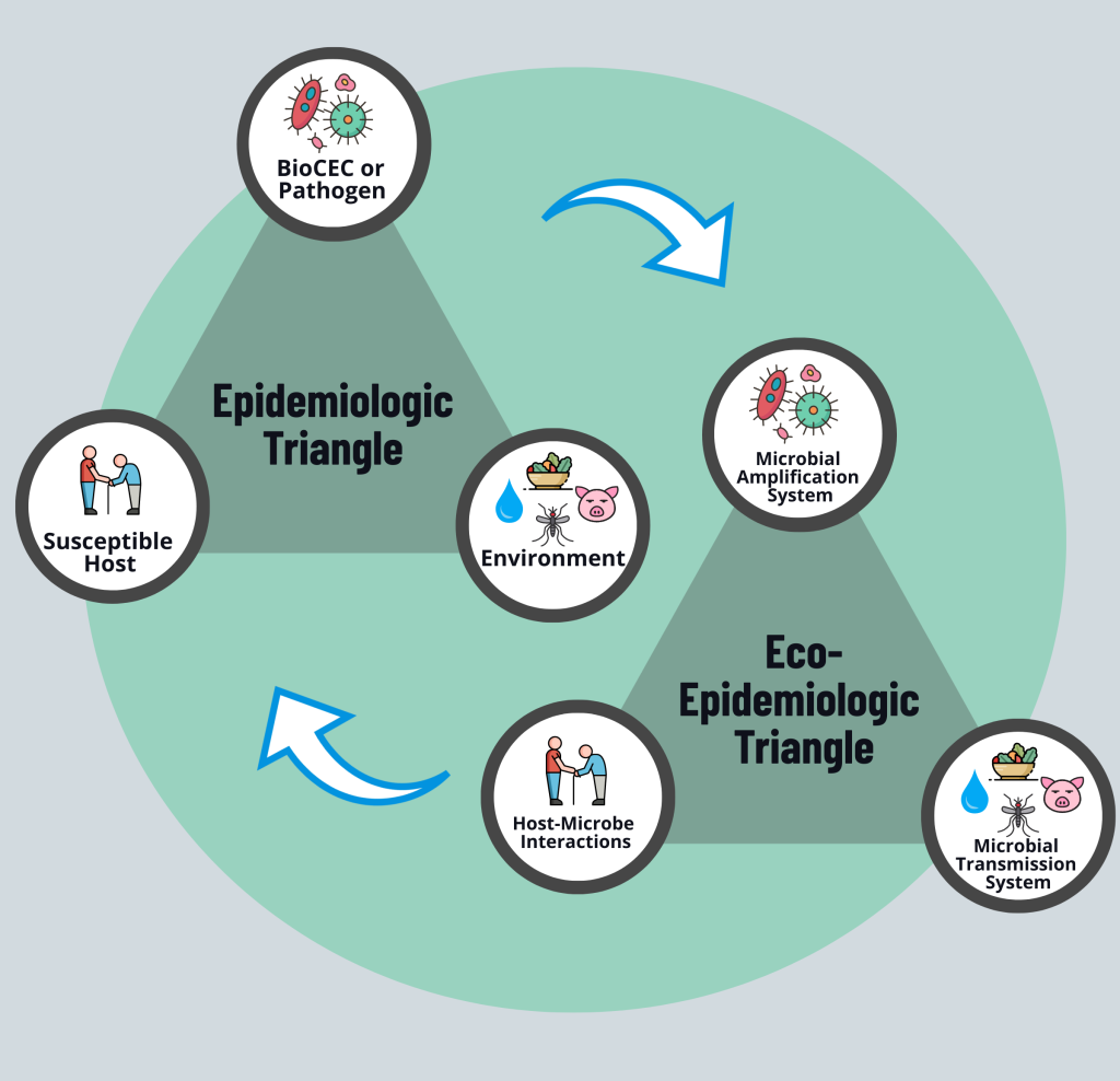
Figure 2. The epidemiologic triangle and the microbiological eco-epidemiologic triangle.
Source: Adapted from (
CDC 2024 [Q9KEGHPZ] CDC. 2024. “About One Health.” One Health, November 21. https://www.cdc.gov/one-health/about/index.html.
).
It is noteworthy that the term ‘environment’ in the epidemiological triangle was used as a general term that applied to any and all factors and determinants of infectious diseases, including socioeconomic and demographic variables ( John and Kompithra 2023 [MWY6GAI7] John, T. Jacob, and Rajeev Zachariah Kompithra. 2023. “Eco-Epidemiology Triad to Explain Infectious Diseases.” Indian Journal of Medical Research 158 (2): 107. https://doi.org/10.4103/ijmr.ijmr_3031_21. ). Some pathogens are directly transmitted from human to human or animal to human. In those cases, the infected host/reservoir/vector is actually the “environment” for the uninfected would-be host in the vicinity. Given the confusion this creates, several epidemiologists and authors have created the eco-epidemiological triangle (see Figure 2), which explains disease transmission in terms of microbial amplification systems, microbial transmission systems, and microbe-host pathogen interactions ( John et al. 2024 [7M5IJL23] John, T. Jacob, Dhanya Dharmapalan, Robert Steinglass, and Norbert Hirschhorn. 2024. “The Role of Adults in Poliovirus Transmission to Infants and Children.” VIEWPOINT. Global Health: Science and Practice 12 (2). https://doi.org/10.9745/GHSP-D-23-00363. ).
Due to the prevalence of concerns regarding the threat of anthroponotic and zoonotic diseases, this document includes some information on these types of diseases. Exposure to pathogens that are vector-borne requires an understanding of other environmental factors (e.g., humidity, rainfall, temperature) that can increase or change the vector population. This section will also cover vector-borne diseases specifically focusing on vectors (mosquitoes, ticks) that are affected by changes in the environment. Certain foodborne diseases will be discussed briefly in this section when the exposure pathway of concern is associated with pathogenic contaminants discovered in farm soil or water used for irrigation.
3. Considerations for Assessing Risks from BioCEC
3.1 Pathogens
Vignette #1. Extracellular vs. Intracellular Pathogens
The distinction between extracellular and intracellular pathogens is increasingly muddled.
It is noteworthy that an increasing number of bacteria, which we had previously described as extracellular (e.g., Pseudomonas aeruginosa, E. coli, Vibrio cholerae, and Acinetobacter baumannii) have documented strains that exhibit facultative intracellular characteristics ( Pirofski and Casadevall 2012 [FZ44SSS5] Pirofski, Liise-anne, and Arturo Casadevall. 2012. “Q&A: What Is a Pathogen? A Question That Begs the Point.” BMC Biology 10 (1): 6. https://doi.org/10.1186/1741-7007-10-6. ). This has resulted in a debate around whether the capacity for intracellular survival may be more common than previously thought ( Casadevall 2008 [NE7678SP] Casadevall, Arturo. 2008. “Evolution of Intracellular Pathogens.” Annual Review of Microbiology 62 (October): 19–33. https://doi.org/10.1146/annurev.micro.61.080706.093305. ). Given the major implications for human health and disease, as well as infection control and treatment, most public health professionals continue to use this classification system.
The first consideration when assessing risk from a BioCEC is whether or not the organism is considered a pathogen. A pathogen is traditionally defined as an organism that can cause disease in a host, with the severity of the disease symptoms being referred to as virulence ( Mara and Horan 2003 [RBY9THLW] Mara, Duncan, and Nigel Horan, eds. 2003. Handbook of Water and Wastewater Microbiology. Academic Press. https://doi.org/10.1016/B978-0-12-470100-7.50047-9. ). A host is an organism that harbors a pathogen or parasite. The outcome of the microbe-host relationship depends on the pathogenicity of the organism and the susceptibility of the host. Pathogens are taxonomically diverse and comprise a broad range of viruses and bacteria, as well as unicellular eukaryotes (e.g., amoeba, algae, protozoa) and multicellular eukaryotes (e.g., fungi) ( Madigan et al. 2021 [MXEA6KXC] Madigan, Michael T., Kelly S. Bender, Daniel H. Buckley, W. Matthew Sattley, David A. Stahl, and Thomas D. Brock. 2021. Brock Biology of Microorganisms. Sixteenth edition, Global edition. Pearson Education Limited. ). All organisms are susceptible to pathogens, including bacteria, which are targeted by specialized viruses called phages. More recently, there has been some debate among researchers that the original definition of pathogenicity is insufficient and that pathogens should be defined as organisms that can cause harm or damage to a host ( Balloux and van Dorp 2017 [WKTVNTAP] Balloux, Francois, and Lucy van Dorp. 2017. “Q&A: What Are Pathogens, and What Have They Done to and for Us?” BMC Biology 15 (1): 91. https://doi.org/10.1186/s12915-017-0433-z. ). There are several ways to categorize pathogens, including by the level of dependence on the host for survival (e.g., intra- vs. extracellular pathogens) or the likelihood of triggering illness (e.g., strict versus opportunistic pathogen). Pathogen classifications tend to overlap and are not mutually exclusive, but they are explained below to provide the reader with clarity on the differences. Some familiarity with pathogen properties will help create a standardized dialogue among microbiologists, epidemiologists, and public health professionals. It also helps explain risk characterization and mitigation strategies to reduce risk.
Vignette #2. Extracellular vs. Intracellular Pathogens
Distinguishing facultative and obligate intracellular parasites.
The classical division between facultative and obligate intracellular parasites has been based on the presence (in facultative intracellular bacteria) or absence (in obligate intracellular bacteria) of the capacity to multiply in a cell-free environment, which is evaluated using artificial bacteriological media ( Silva and Silva Pestana 2013 [QCI7B5LP] Silva, Manuel T., and Nazaré T. Silva Pestana. 2013. “The in Vivo Extracellular Life of Facultative Intracellular Bacterial Parasites: Role in Pathogenesis.” Immunobiology 218 (3): 325–37. https://doi.org/10.1016/j.imbio.2012.05.011. ). Obligate intracellular bacteria cannot be grown in artificial media (agar plates/broths) in laboratories because they require viable eukaryotic host cells (e.g., cell culture, embryonated eggs, and susceptible animals). For example, Chlamydia trachomatis is an obligate intracellular bacterium. Chlamydial cells depend on the host cell for adenosine triphosphate and other intermediate molecule production because they are unable to carry out energy metabolism and lack many biosynthetic pathways.
3.1.1 Intra- and Extracellular Pathogens
Classically, infectious agents have been classified as extracellular, facultative intracellular, and obligate intracellular pathogens ( Leon-Sicairos et al. 2015 [DGCK65EJ] Leon-Sicairos, Nidia, Ruth Reyes-Cortes, Alma M. Guadrón-Llanos, Jesús Madueña-Molina, Claudia Leon-Sicairos, and Adrian Canizalez-Román. 2015. “Strategies of Intracellular Pathogens for Obtaining Iron from the Environment.” BioMed Research International 2015 (1): 476534. https://doi.org/10.1155/2015/476534. ). This has major implications for how the pathogen replicates and enters the host (i.e., how risk can be mitigated), whether immunity can be developed, and whether medication can be effective against the pathogen.
Staphylococcus aureus, Pseudomonas aeruginosa, Streptococcus pyogenes and most E. coli strains are examples of extracellular pathogenic bacteria that need a “portal of entry” or “transmission route” to enter the host, and they cause a range of infections. These organisms usually have the capacity to survive and sometimes replicate in the environment outside of the host ( Silva 2012 [WGK8GBJZ] Silva, Manuel T. 2012. “Classical Labeling of Bacterial Pathogens According to Their Lifestyle in the Host: Inconsistencies and Alternatives.” Frontiers in Microbiology 3 (February). https://doi.org/10.3389/fmicb.2012.00071. ), which has implications for the CEM, microbial transmission, and the amplification systems in the eco-epidemiological triangle.
Transmission routes to reach the site of injury or infection include water, air, wound, food, mechanical vectors, and fomite contact. Once arrived, these pathogens multiply in the host at extracellular sites or outside of cells (e.g., mucosal surfaces; interstitial spaces; or vascular, lymphatic, or body cavity fluids) ( Silva and Silva Pestana 2013 [QCI7B5LP] Silva, Manuel T., and Nazaré T. Silva Pestana. 2013. “The in Vivo Extracellular Life of Facultative Intracellular Bacterial Parasites: Role in Pathogenesis.” Immunobiology 218 (3): 325–37. https://doi.org/10.1016/j.imbio.2012.05.011. ) to cause damage and use virulence mechanisms to evade the immune system, thus promoting extracellular multiplication ( Leon-Sicairos et al. 2015 [DGCK65EJ] Leon-Sicairos, Nidia, Ruth Reyes-Cortes, Alma M. Guadrón-Llanos, Jesús Madueña-Molina, Claudia Leon-Sicairos, and Adrian Canizalez-Román. 2015. “Strategies of Intracellular Pathogens for Obtaining Iron from the Environment.” BioMed Research International 2015 (1): 476534. https://doi.org/10.1155/2015/476534. ).
Intracellular survival is considered an evolutionary strategy that decreases competition between the pathogen and other organisms and improves chances of avoiding predation by amoeba in the environment (i.e., survival inside predator amoeba similar to Legionella and Campylobacter) resulting in endosymbiotic existence within protozoa ( Casadevall 2008 [NE7678SP] Casadevall, Arturo. 2008. “Evolution of Intracellular Pathogens.” Annual Review of Microbiology 62 (October): 19–33. https://doi.org/10.1146/annurev.micro.61.080706.093305. ). Intracellular pathogens must enter into host cells to survive and reproduce (e.g., macrophages, epithelial cells), which makes them especially relevant from a public health perspective and difficult to eradicate ( Silva and Silva Pestana 2013 [QCI7B5LP] Silva, Manuel T., and Nazaré T. Silva Pestana. 2013. “The in Vivo Extracellular Life of Facultative Intracellular Bacterial Parasites: Role in Pathogenesis.” Immunobiology 218 (3): 325–37. https://doi.org/10.1016/j.imbio.2012.05.011. Silva 2012 [WGK8GBJZ] Silva, Manuel T. 2012. “Classical Labeling of Bacterial Pathogens According to Their Lifestyle in the Host: Inconsistencies and Alternatives.” Frontiers in Microbiology 3 (February). https://doi.org/10.3389/fmicb.2012.00071. Pirofski and Casadevall 2012 [FZ44SSS5] Pirofski, Liise-anne, and Arturo Casadevall. 2012. “Q&A: What Is a Pathogen? A Question That Begs the Point.” BMC Biology 10 (1): 6. https://doi.org/10.1186/1741-7007-10-6. Leon-Sicairos et al. 2015 [DGCK65EJ] Leon-Sicairos, Nidia, Ruth Reyes-Cortes, Alma M. Guadrón-Llanos, Jesús Madueña-Molina, Claudia Leon-Sicairos, and Adrian Canizalez-Román. 2015. “Strategies of Intracellular Pathogens for Obtaining Iron from the Environment.” BioMed Research International 2015 (1): 476534. https://doi.org/10.1155/2015/476534. ). Moreover, once inside host cells, they use specific pathways to evade the adaptive immune response to survive and replicate within host cells, as they are not directly accessible to antibodies, and their persistence relies on evading cell-mediated immunity. An example of this is Legionella pneumophila, which prefers the intracellular environment of macrophages for growth and blocks host destructive enzymes inside cells.
Obligate intracellular bacteria include Coxiella burnetii, Rickettsia spp.; certain protozoa such as Trypanosoma spp., Plasmodium, and Toxoplasma; fungi such as Pneumocystis jirovecii; all viruses and many vector-borne pathogens ( Silva and Silva Pestana 2013 [QCI7B5LP] Silva, Manuel T., and Nazaré T. Silva Pestana. 2013. “The in Vivo Extracellular Life of Facultative Intracellular Bacterial Parasites: Role in Pathogenesis.” Immunobiology 218 (3): 325–37. https://doi.org/10.1016/j.imbio.2012.05.011. Silva 2012 [WGK8GBJZ] Silva, Manuel T. 2012. “Classical Labeling of Bacterial Pathogens According to Their Lifestyle in the Host: Inconsistencies and Alternatives.” Frontiers in Microbiology 3 (February). https://doi.org/10.3389/fmicb.2012.00071. Leon-Sicairos et al. 2015 [DGCK65EJ] Leon-Sicairos, Nidia, Ruth Reyes-Cortes, Alma M. Guadrón-Llanos, Jesús Madueña-Molina, Claudia Leon-Sicairos, and Adrian Canizalez-Román. 2015. “Strategies of Intracellular Pathogens for Obtaining Iron from the Environment.” BioMed Research International 2015 (1): 476534. https://doi.org/10.1155/2015/476534. ). When intra-cellularity is transient, the organism is considered a facultative intracellular pathogen (e.g., Francisella tularensis, Listeria monocytogenes, Salmonella typhi, Mycobacterium spp.). These are capable of living and reproducing either inside or outside host cells, making their lifestyles more adaptive ( Leon-Sicairos et al. 2015 [DGCK65EJ] Leon-Sicairos, Nidia, Ruth Reyes-Cortes, Alma M. Guadrón-Llanos, Jesús Madueña-Molina, Claudia Leon-Sicairos, and Adrian Canizalez-Román. 2015. “Strategies of Intracellular Pathogens for Obtaining Iron from the Environment.” BioMed Research International 2015 (1): 476534. https://doi.org/10.1155/2015/476534. ).
3.1.2 Strict and Opportunistic (or Facultative) Pathogens
Vignette #3. Opportunistic Pathogens
What makes opportunistic pathogens different?
Berg et al. ( Berg et al. 2014 [4CQQPJTI] Berg, Gabriele, Armin Erlacher, Kornelia Smalla, and Robert Krause. 2014. “Vegetable Microbiomes: Is There a Connection among Opportunistic Infections, Human Health and Our ‘Gut Feeling’?” Microbial Biotechnology 7 (6): 487–95. https://doi.org/10.1111/1751-7915.12159. ) suggested that most opportunistic pathogens will have one or more of the following features:
- They elicit antagonistic activity against other microorganisms.
- They are versatile in terms of nutritional needs.
- They are cultivable.
- They are copiotrophs (i.e., organisms that thrive in environments with abundant nutrients, particularly carbon).
- They are highly competitive.
- They are able to form biofilms.
- They can be hypermutators.
- They often have antibiotic and toxin resistance.
The authors hypothesized that more species of opportunistic pathogens will emerge as superbugs in the future since most of these characteristics are strain-specific and acquired through horizontal gene transfer.
Opportunistic or facultative pathogens are organisms for which the host is only one of the potential niches they can exploit to reproduce ( Balloux and van Dorp 2017 [WKTVNTAP] Balloux, Francois, and Lucy van Dorp. 2017. “Q&A: What Are Pathogens, and What Have They Done to and for Us?” BMC Biology 15 (1): 91. https://doi.org/10.1186/s12915-017-0433-z. ). They usually do not cause disease in healthy hosts and are primarily environmental bacteria, parasites, or fungi that can occasionally cause infection when the right conditions present themselves ( Haas et al. 2014 [78R697XZ] Haas, Charles N., Joan B. Rose, and Charles P. Gerba. 2014. “Quantitative Microbial Risk Assessment, 2nd Edition | Wiley.” Wiley.Com. https://www.wiley.com/en-us/Quantitative+Microbial+Risk+Assessment%2C+2nd+Edition-p-9781118910030. ). This has implications for the susceptible population and controls of pathogen in the environment to mitigate risk. In addition, many of the characteristics that lead to the success of opportunistic pathogens in colonizing hosts were properties initially necessary for their survival in the natural habitat (e.g., enhanced resistance to phagocytosis, resistance to irradiation or disinfection) ( De Hoog et al. 2024 [C342W9P8] De Hoog, Sybren, Chao Tang, Xin Zhou, et al. 2024. “Fungal Primary and Opportunistic Pathogens: An Ecological Perspective.” FEMS Microbiology Reviews 48 (5): fuae022. https://doi.org/10.1093/femsre/fuae022. ). An example is biofilm formation. Biofilm formation is a catalyst for persistence and resistance to antimicrobials and changing environmental conditions that would otherwise result in pathogen elimination ( WHO and International Water Association 2009 [N3SWAM7S] WHO, and International Water Association. 2009. Water safety plan manual: step-by-step risk management for drinking-water suppliers. World Health Organization. https://iris.who.int/handle/10665/75141. Singh et al. 2021 [TMBT4KMM] Singh, Shivani, Saptashwa Datta, Kannan Badri Narayanan, and K. Narayanan Rajnish. 2021. “Bacterial Exo-Polysaccharides in Biofilms: Role in Antimicrobial Resistance and Treatments.” Journal of Genetic Engineering and Biotechnology 19 (1): 140. https://doi.org/10.1186/s43141-021-00242-y. Palmer et al. 2007 [PLG5WWR9] Palmer, Jon, Steve Flint, and John Brooks. 2007. “Bacterial Cell Attachment, the Beginning of a Biofilm.” Journal of Industrial Microbiology and Biotechnology 34 (9): 577–88. https://doi.org/10.1007/s10295-007-0234-4. Flemming and Wuertz 2019 [XT89STS9] Flemming, Hans-Curt, and Stefan Wuertz. 2019. “Bacteria and Archaea on Earth and Their Abundance in Biofilms.” Nature Reviews Microbiology 17 (4): 247–60. https://doi.org/10.1038/s41579-019-0158-9. ). Meanwhile, obligate pathogens require a host to fulfill their life cycle (i.e., stages of development of the parasite or pathogen until it reaches its mature infectious stage).
All viruses are obligate pathogens since they require the host’s cell for their reproduction. Obligate pathogens are found among bacteria, including the agents of tuberculosis and syphilis, as well as protozoans (such as those causing malaria) and macroparasites ( Balloux and van Dorp 2017 [WKTVNTAP] Balloux, Francois, and Lucy van Dorp. 2017. “Q&A: What Are Pathogens, and What Have They Done to and for Us?” BMC Biology 15 (1): 91. https://doi.org/10.1186/s12915-017-0433-z. ). Some obligate pathogens require multiple hosts to complete their life cycle. The definite host, which supports the adult form of the pathogen, is often a vertebrate, and the intermediate host (referred to as a vector) is generally an arthropod or a mollusk. This alternation of vertebrate and invertebrate hosts is found in viruses (for example the Zika virus), bacteria (for example Lyme disease), and protozoa (malaria). Trematodes (parasitic flatworms or platyhelminths) go even further and require two or more intermediate hosts ( Roberts et al. 2012 [6CYZYZAR] Roberts, Larry S., John J. Janovy, and Steve Nadler. 2012. Foundations of Parasitology. McGraw-Hill Education. ).
Vignette #4. Biofilms
How relevant are biofilms to CEM development and risk assessment?
Biofilms are complex communities of attached microorganisms that are bound to biotic or abiotic surfaces by polysaccharides, proteins, and nucleic acids. This slimy matrix surrounding the cells is called an extracellular polymeric substance, and it creates a barrier that reduces susceptibility to environmental changes, disinfectants, and antibiotics. The extracellular polymeric substance also allows for concentration of nutrients, protection from phagocytosis and predation, extracellular enzyme usage by cells that cannot produce those enzymes, and increased horizontal gene transfer and retention of mobile genetic elements. Biofilm development leads to the formation of complex structures important for disease development, infection control, and engineering applications. Bacteria are far more likely to be found in biofilms in the natural environment than in planktonic (free- living) form.
When BioCEC require intermediate hosts, understanding all the components of the life cycle helps in the evaluation of infection control measures. For example, knowing that swimmer’s itch (or cercarial dermatitis) requires a life cycle stage in snails and then in birds allows public health officials to implement the right tools for monitoring, controlling, and eradicating the cause. It also helps in the development of an accurate CEM as seen in the Conceptual Exposure Model.
Vignette #5. Host Microbe Interactions
How specific is the site of infection within the host?
The host contains a diverse range of niches that pathogens can colonize and inhabit, since each region within the host is physically and chemically distinct. The microbiomes of skin, the respiratory tract, and the gastrointestinal tract are highly diverse. The highly oxygenated environment of the lungs favors obligate aerobes, such as Mycobacterium tuberculosis. The dry nature of skin selects for desiccation-resistant Staphylococcus aureus. Meanwhile, the anoxic environment of the large intestines selects for obligate anaerobic bacteria, such as Bacteroides and Clostridium ( Madigan et al. 2021 [MXEA6KXC] Madigan, Michael T., Kelly S. Bender, Daniel H. Buckley, W. Matthew Sattley, David A. Stahl, and Thomas D. Brock. 2021. Brock Biology of Microorganisms. Sixteenth edition, Global edition. Pearson Education Limited. ). More detail on these processes are provided in supplementary material. The following sections on host-microbe interactions are adapted from Brock’s Microbiology ( Madigan et al. 2021 [MXEA6KXC] Madigan, Michael T., Kelly S. Bender, Daniel H. Buckley, W. Matthew Sattley, David A. Stahl, and Thomas D. Brock. 2021. Brock Biology of Microorganisms. Sixteenth edition, Global edition. Pearson Education Limited. ). Regardless of the final site of infection, the pathogen has to gain access to and infect the host tissue. This includes four distinct stages: entry, survival, replication, and exit from the host cell. These stages are shown in Figure 3, along with other bacterial pathogen characteristics ( Silva and Silva Pestana 2013 [QCI7B5LP] Silva, Manuel T., and Nazaré T. Silva Pestana. 2013. “The in Vivo Extracellular Life of Facultative Intracellular Bacterial Parasites: Role in Pathogenesis.” Immunobiology 218 (3): 325–37. https://doi.org/10.1016/j.imbio.2012.05.011. ).
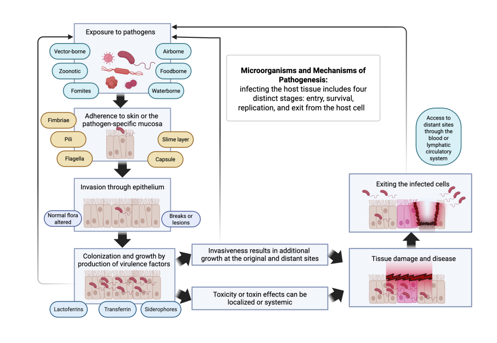
Source: Adapted from ( Madigan et al. 2021 [MXEA6KXC] Madigan, Michael T., Kelly S. Bender, Daniel H. Buckley, W. Matthew Sattley, David A. Stahl, and Thomas D. Brock. 2021. Brock Biology of Microorganisms. Sixteenth edition, Global edition. Pearson Education Limited. ).
Vignette #6. Infective Dose and Virulence
How do we know what the infective dose of a pathogens is?
The infective dose can be estimated by the use of human challenge studies, outbreaks or ‘natural experiments,’ or a combination of both ( Teunis 2022 [MK33MVAE] Teunis, Peter F. M. 2022. “Dose Response for Salmonella typhimurium and Enteritidis and Other Nontyphoid Enteric Salmonellae.” Epidemics 41 (December): 100653. https://doi.org/10.1016/j.epidem.2022.100653. ). Human challenge studies, or dose–response experiments, with healthy adult volunteers can be used to determine the probability of infection at different dose levels. Although these studies are typically regarded as the “gold standard,” for determination of a dose-response assessment, they are ethically restricted to less virulent pathogenic strains and to healthy adult populations. Additionally, these studies often have limited sample sizes. Alternatively, the use of outbreak investigation data is helpful for mimicking “real-world” conditions. Outbreaks may, however, introduce bias by selecting for more susceptible hosts.
3.1.3 Infective Dose
The ability of an infectious disease to cause illness depends on the concentration of the microorganism in the environment the host is exposed to, the infective dose of the pathogen, and the virulence of the pathogen ( Ekdahl et al. 2005 [R6SDSNLN] Ekdahl, Karl, Bengt Normann, and Yvonne Andersson. 2005. “Could Flies Explain the Elusive Epidemiology of Campylobacteriosis?” BMC Infectious Diseases 5 (1): 11. https://doi.org/10.1186/1471-2334-5-11. ). It is commonly believed that the infective dose refers to a minimum threshold value above which infection occurs. In reality, the infective dose characterizes the probability of infection by providing the dose of pathogens above which the probability of infection exceeds a certain value.
The probability of illness to develop from an infection depends upon the degree of host damage (which can be influenced by age/life stage, preexisting illnesses, and factors that may make the host vulnerable or susceptible to damage) and whether this is sufficient to result in clinical symptoms ( Bridle 2021 [LZCVB2TP] Bridle, Helen. 2021. “Chapter 2 — Overview of Waterborne Pathogens.” In Waterborne Pathogens (Second Edition), edited by Helen Bridle. Academic Press. https://doi.org/10.1016/B978-0-444-64319-3.00002-2. Madigan et al. 2021 [MXEA6KXC] Madigan, Michael T., Kelly S. Bender, Daniel H. Buckley, W. Matthew Sattley, David A. Stahl, and Thomas D. Brock. 2021. Brock Biology of Microorganisms. Sixteenth edition, Global edition. Pearson Education Limited. ).
Overall, studies suggest that different groups of pathogens have different infective doses and levels of persistence. An example is provided in Table 1. The WHO considers the relative infectivity as low if the infective dose is greater than 104 pathogens, moderate for doses between 102 and 104, and high for doses between 1 and 102. There is no indication in the WHO list of what probability of infection this infective dose represents ( Bridle 2021 [LZCVB2TP] Bridle, Helen. 2021. “Chapter 2 — Overview of Waterborne Pathogens.” In Waterborne Pathogens (Second Edition), edited by Helen Bridle. Academic Press. https://doi.org/10.1016/B978-0-444-64319-3.00002-2. ).
Humans can acquire infectious diseases even through exposure to very low levels of infectious particles. For example, an infectious dose of influenza A to humans is very low and is believed to be acquired through airborne and droplet means, whereas the infectious dose for Francisella tularensis is reported to be a single organism. Only a few cells of Mycobacterium tuberculosis are required to overcome normal lung clearance and inactivation mechanisms in a susceptible host ( Cole and Cook 1998 [PPYWULGY] Cole, Eugene C., and Carl E. Cook. 1998. “Characterization of Infectious Aerosols in Health Care Facilities: An Aid to Effective Engineering Controls and Preventive Strategies.” American Journal of Infection Control 26 (4): 453–64. https://doi.org/10.1016/S0196-6553(98)70046-X. ). The dose required for Salmonella spp. is influenced by the nature and physiological status of the strain, the matrix in which the strain is ingested, and the status of the potential host. Although the “typical” infectious dose is considered to be about 106–108 colony-forming units, epidemiological outbreak data suggest that the infectious dose can be substantially less, as little as a few cells ( Cox and Pavic 2014 [IM5UTA3I] Cox, J. M., and A. Pavic. 2014. “SALMONELLA | Introduction.” In Encyclopedia of Food Microbiology (Second Edition), edited by Carl A. Batt and Mary Lou Tortorello. Academic Press. https://doi.org/10.1016/B978-0-12-384730-0.00294-9. ).
Table 1. General characteristics of enteric pathogens and their impact on causing infections through water reuse
| Pathogen Type | Persistence in the Environment | Minimum Infective Dose | Immunity | Life Cycle Development in the Environment | Opportunistic or Strict Pathogen |
| Viruses | Medium | Low | Long | No | Strict |
| Bacteria | Short to medium | Medium–high | Short to medium | No | Both |
| Protozoa | Medium | Low–medium | None/little | No | Both |
| Helminths | Long | Low | None/little | Yes | Both |
Source: Adapted from ( Mara and Horan 2003 [RBY9THLW] Mara, Duncan, and Nigel Horan, eds. 2003. Handbook of Water and Wastewater Microbiology. Academic Press. https://doi.org/10.1016/B978-0-12-470100-7.50047-9. ).
Vignette #7. Infective Dose and Virulence
How do bacterial pathogens enter and colonize host cells?
In most cases reaching the hosts site of infection requires that the pathogen penetrate surfaces that would usually be considered barriers to infection (e.g., skin, mucous membranes, intestinal epithelium). Most microbial infections begin at breaks in the skin (e.g., cuts, wounds) or possibly lesions in the mucous membranes of the respiratory, digestive, or genito-urinary tract. Epithelial tissue attachment requires macromolecular interactions on the surfaces of both the pathogen and the host cell (e.g., binding to specific cell surface proteins). The attachment tends to be fairly selective, and pathogens do not adhere to all epithelial cells equally. In addition, adhesion strength can be fairly host specific, so that attachment in the correct final host is stronger, influencing host range where successful colonization and infection can occur. Attachment to host cells can be accomplished through slime layers, capsules, fimbriae, and pili. In addition, some bacteria produce enzymes and toxins to initiate pathogenicity.
Some macromolecules responsible for bacterial attachment are not covalently attached to the bacteria (e.g., polysaccharides, proteins, protein-carbohydrate mixtures) but secreted by bacteria. This loose network of polymeric fibers extending outward from the cell is called a slime layer. A polymer coat consisting of a dense, well-defined layer surrounding the cell is called a capsule. These structures are not just important for attachment to the host but may also influence interactions with surfaces and attachment to other bacteria.
Fimbriae and pili are bacterial cell surface structures that may also influence cell surface protein structures critical to the attachment process. Among the most detailed descriptions of fimbriae are the Type I fimbriae of enteric bacteria, which are uniformly distributed on the cell surface (e.g., Escherichia, Klebsiella, Salmonella, Shigella). Pili are typically longer than fimbriae, fewer in number, and are found on the surface of the cell. Both pili and fimbriae function by binding to host cell surface glycoproteins, initiating attachment. Flagella are also known to improve attachment to host cells.
To accomplish invasion, pathogens must penetrate the epithelium to initiate pathogenicity. Toxin-producing bacteria are the exception to this rule, and do not need to invade the host cell. Growth can occur after entry through a lesion in the mucosal membrane or on the surface if the microflora of the epithelium is altered enough. Pathogens then colonize the tissue and potentially grow in numbers or expand to more distant sites within the host through the blood or lymphatic circulation systems.
Enzymes can promote spreading of the organism by breaking down molecules that act like physical barriers to spread (e.g., streptococci and staphylococci produce hyaluronidase, which breaks down the polysaccharide hyaluronic acid that acts like an extracellular cement between animal cells).
Enzymes (e.g., proteases, lipases, nucleases) can break down intracellular host cell enzymes and disrupt basic functions. Some enzymes (e.g., collagenase produced by clostridia) disrupt the collagen network supporting host tissue, thereby allowing spread through the body.
Some pathogens produce enzymes that produce fibrin clots (e.g., coagulase produced by S. aureus cells) at the site of infection to localize and protect the organism. Coagulase also helps deposit fibrin inside the S. aureus cells to protect it from host cell attacks.
Vignette #8. Determining LD50
How do toxicologists determine an LD50?
Toxicologists can use many kinds of animals, but most often testing is done with rats and mice. It is usually expressed as the amount of chemical administered (e.g., milligrams) per 100 grams (for smaller animals) or per kilogram body weight of the test animal (for larger test subjects). An LD50 can be determined for dermal contact (applied to the skin) and oral (given by mouth) administration methods ( Canadian Centre for Occupational Health and Safety 2025 [I59GPPY6] Canadian Centre for Occupational Health and Safety. 2025. “CCOHS: Chemicals and Materials.” April 15. https://www.ccohs.ca/oshanswers/chemicals. ). This is different from the Lethal Concentration50, which specifically refers to the concentration of a chemical in air or water.
3.1.4 Virulence
Virulence is the degree of severity or harmfulness of a disease caused by a pathogen ( Madigan et al. 2021 [MXEA6KXC] Madigan, Michael T., Kelly S. Bender, Daniel H. Buckley, W. Matthew Sattley, David A. Stahl, and Thomas D. Brock. 2021. Brock Biology of Microorganisms. Sixteenth edition, Global edition. Pearson Education Limited. ). It is in part enabled by the organism’s toxicity and invasiveness. Virulence factors are bacterial components or molecules that enable a pathogen to establish itself, evade the immune system, and cause disease by enhancing its ability to attach to host cells, damage tissues, and/or produce toxins.
Virulence is estimated from experimental studies of the lethal dose50 (LD50). The LD50 is the single dose of an organism, compound, or substance that is expected to kill 50% of a group of test animals in a laboratory setting. The LD50 dose is usually expressed as milligrams or grams of material per kilogram of animal body weight (mg/kg or g/kg).
For highly virulent pathogens, the dose it takes to kill 50% of the population may be only slighter lower than the dose it takes to kill 100%, making exposure reduction crucial. Only a few cells of the highly virulent Streptococcus pneumoniae are required to establish a fatal infection and kill all animals in a test population. In comparison, the LD50 of the moderately virulent Salmonella typhimurium is much higher, and the number of cells of S. typhimurium needed to kill 100% of the population is almost 100 times higher than the organism’s LD50 ( Madigan et al. 2021 [MXEA6KXC] Madigan, Michael T., Kelly S. Bender, Daniel H. Buckley, W. Matthew Sattley, David A. Stahl, and Thomas D. Brock. 2021. Brock Biology of Microorganisms. Sixteenth edition, Global edition. Pearson Education Limited. ).
Vignette #9. Strains: Phenotypes Vs. Genotypes
How are phenotype and genotype different?
Genotype is determined solely using genetic information dictating specific traits, whereas microbial phenotype specifically looks at the expressed (i.e., visible) traits of organisms, which are influenced both by both genetic determinants and environmental factors (Wiedmann 2019). Assessing strain virulence through “observed” variability at the phenotype level provides helpful information to assess other relevant factors, including stress resistance, distribution, virulence, and epidemiology of the pathogenic organism. Moreover, with particular reference to foodborne pathogens, it has been acknowledged that intra-species variability may have an important impact on the accuracy of microbiological risk assessment ( Lianou et al. 2020 [CU6XNX8P] Lianou, Alexandra, George-John E. Nychas, and Konstantinos P. Koutsoumanis. 2020. “Strain Variability in Biofilm Formation: A Food Safety and Quality Perspective.” Food Research International 137 (November): 109424. https://doi.org/10.1016/j.foodres.2020.109424. ). It is important to know that virulent strains kept in laboratory cultures, as opposed to isolation from diseased animals, undergo attenuation, which is a decrease or loss of virulence. Non-virulent or weakly virulent mutants are subject to faster growth and thus end up being selectively favored and outcompeting highly pathogenic strains. Attenuated strains are often used for vaccine production.
Essential bacterial genes orchestrate core biological processes and represent the targets of nearly all antibacterial drugs ( Bosch et al. 2021 [GMX85JDU] Bosch, Barbara, Michael A. DeJesus, Nicholas C. Poulton, et al. 2021. “Genome-Wide Gene Expression Tuning Reveals Diverse Vulnerabilities of M. tuberculosis.” Cell 184 (17): 4579-4592.e24. https://doi.org/10.1016/j.cell.2021.06.033. ). While genotyping determines the differences in the genetic makeup of the pathogen by examining the individual organism’s DNA or RNA sequences using molecular tools, having a gene does not necessitate its expression or activity. Genes can be up- or downregulated. Partial inhibition of some essential genes results in decreased bacterial fitness, whereas other essential genes can tolerate substantial inhibition with little effect on bacterial fitness. This expression–fitness relationship is defined as gene vulnerability. Gene vulnerability relates the magnitude of gene expression inhibition with the resulting decrease in organismal fitness, thus describing gene essentiality as a continuous trait ( Bosch et al. 2021 [GMX85JDU] Bosch, Barbara, Michael A. DeJesus, Nicholas C. Poulton, et al. 2021. “Genome-Wide Gene Expression Tuning Reveals Diverse Vulnerabilities of M. tuberculosis.” Cell 184 (17): 4579-4592.e24. https://doi.org/10.1016/j.cell.2021.06.033. ).
When referring to virulence, the term strain variability is often used to describe the inherent differences among identically treated strains of the same microbial species. Historically, strain has meant a microbial isolate, although the definition is not well-suited to microbial community studies. Now, the term is used to refer to a specific microbial genome or collection of clonally identical cells (i.e., a genotype); one or more colonies (believed to be) derived from the same progenitor cell; or most often, in practice, a collection of cells or genomes within a relatively small range of phylogenetic variation (i.e., a very narrow subspecies clade) ( Yan et al. 2020 [NFSA7SD7] Yan, Yan, Long H. Nguyen, Eric A. Franzosa, and Curtis Huttenhower. 2020. “Strain-Level Epidemiology of Microbial Communities and the Human Microbiome.” Genome Medicine 12 (1): 71. https://doi.org/10.1186/s13073-020-00765-y. ). Given this definition, to differentiate pathogens beyond the species level (i.e., strain typing or subtyping), genotypic or phenotypic characteristics are used ( Lianou et al. 2020 [CU6XNX8P] Lianou, Alexandra, George-John E. Nychas, and Konstantinos P. Koutsoumanis. 2020. “Strain Variability in Biofilm Formation: A Food Safety and Quality Perspective.” Food Research International 137 (November): 109424. https://doi.org/10.1016/j.foodres.2020.109424. ).
Extracellular capsules, slime layers, cell walls, envelopes, fimbriae, and pili are all integral to a pathogen’s ability to produce infection, act as virulence factors, and are somewhat distinct from other intra and extracellular components that function solely as virulence factors with similar modes of action — for example, exotoxins (e.g., enterotoxins) and endotoxins enzymes. A broad range of toxins that pathogens can produce are considered virulence factors. Toxins are divided into two categories: exotoxins (e.g., enterotoxins) and endotoxins.
3.2 Environment
The environment is a key factor in understanding the spread and potential adverse effects of BioCEC. An environment can be characterized by scale, time, and geographic or biological location. A geographic location and the population living within it have a reciprocal relationship. Socioeconomic factors describe a population’s income, occupation, education, living conditions, opportunity, and resources while geographic factors describe a location’s landforms, natural resources, climate, and built environment. Both geographic location and socioeconomic factors play a large role in a BioCEC event by impacting factors such as population distribution, urbanization, behavior, travel of people and goods, industry, and extent of regulatory involvement. Biofilms that occur in engineered environments such as wastewater treatment plants, water reuse systems, and distribution infrastructure could differ from biofilms and pathogen occurrence in natural environments in non-developed or non-urbanized settings. The proper control and operation of engineered environments limits human exposure to pathogens. Environment is a broad term that can be used to describe the human body as an environment or a geographical region, such as an estuary or the Southeastern United States. Human environments are characterized by differences in cultural, physical, and biological conditions. Rapid growth in a human population or behavioral patterns such as frequent travel over long distances can affect the prevalence and potential of exposure to pathogens. A thorough consideration of the environment where a pathogen and host might interact helps to assess the risk of illness ( Craun et al. 2010 [AFD7C3LS] Craun, Gunther F., Joan M. Brunkard, Jonathan S. Yoder, et al. 2010. “Causes of Outbreaks Associated with Drinking Water in the United States from 1971 to 2006.” Clinical Microbiology Reviews 23 (3): 507–28. https://doi.org/10.1128/CMR.00077-09. WHO 2025 [APWV7C7K] WHO. 2025. “World Health Organization (WHO).” https://www.who.int. ).
It is important to consider environmental variables that affect pathogens and potential hosts as well as vector populations. Some pathogens survive in multiple media, although they might only flourish and multiply in one medium. Similarly, certain pathogens thrive within a particular temperature range, although they might survive outside their preferred conditions. An environment that is conducive to survival and multiplication of a pathogen will lend itself to generating a sufficient concentration to infect a host. Other considerations include antibiotic-resistance genes that can be a cofactor for pathogen virulence and epigenetics, which result in changes to how genes work, thus potentially impacting the vulnerability of a host to a pathogen. Stressors other than potential BioCEC might be present, such as chemical contamination or physical stressors such as heat or even psychological stressors associated with events like natural disasters. Although waterborne transmission of disease is well documented, pathogens can be transmitted by other media including soil and air ( Craun et al. 2010 [AFD7C3LS] Craun, Gunther F., Joan M. Brunkard, Jonathan S. Yoder, et al. 2010. “Causes of Outbreaks Associated with Drinking Water in the United States from 1971 to 2006.” Clinical Microbiology Reviews 23 (3): 507–28. https://doi.org/10.1128/CMR.00077-09. ).
The WHO’s website provides information about how environment influences the spread of diseases. The prevalence of pathogens can increase depending upon local climate conditions. Weather events such as flooding can lead to spillage from sewage systems or damage to systems that provide clean drinking water.
Environmental factors vary widely from place to place and with time. The following list provides examples of environmental factors that can affect risk of exposure and infection from BioCEC:
- Anthropogenic activity
- Waste disposal or reuse (impoundments, landfills, biosolid applications)
- Waste release
- Solid waste landfills
- Sewage/septic tank (domestic waste)
- Medical waste, animal waste
- Land disposal of fecal-contaminated solid waste (diapers)
- Agriculture (crops and livestock)
- Produce farming
- Biosolids (Class B) application
- Recycled water (non-potable reuse and potable reuse)
- Animal feeding operations or agricultural animal production
- Infrastructure and urban operations
- Water supply and treatment
- Cooling towers, plumbing, etc.
- Treatment: for example, water disinfection, removal/inactivation, failures in treatment barriers
- Waste disposal or reuse (impoundments, landfills, biosolid applications)
- Geography and weather
- Seasonality
- Events that depart from historical norms
- Events exacerbated by climate change:
- Wildfires
- Seawater intrusion into coastal aquifers and water distribution lines
- Algal blooms
- Reemergence of microbes from permafrost
- Multiple factors that affect pathogen survival in the environment: temperature, moisture, pH, organic matter, native microbial flora
- Vector characteristics
- Characteristics particular to thriving in the environment
- Ability to infect human receptors
- Factors that affect vector population density
- Reservoir and intermediate hosts
- Transported as aerosols/airborne droplets
As the list above implies, environmental factors can be divided into multiple categories. The WHO summarizes the most important environmental factors as water supply, sanitation facilities, food, and climate. When there is disruption associated with these environmental variables, the potential for risk of exposure and infection can increase.
3.3 Host
In this subsection, the host refers to a human that is exposed to or harbors pathogenic agents found in the environment. A host can manifest the symptoms and health effects or show no symptoms (carrier or subclinical infection). The observation of health effects may also depend on the incubation period (from time of exposure until symptoms appear) or duration of the clinical spectrum of the disease. Transmission of pathogens from the environmental media (e.g., waterborne, airborne, soil) to the human host will be the focus of this section. Information on human host as a source of emerging BioCEC, such as human-to-human direct transmission, will not be covered in this section; information on infectious diseases due to human-to-human transmissions (e.g., influenzas) can be found on the CDC ( CDC 2025 [PN93EYZ4] CDC. 2025. “Centers for Disease Control and Prevention.” March 31. https://www.cdc.gov/index.html. ) and WHO ( WHO 2025 [APWV7C7K] WHO. 2025. “World Health Organization (WHO).” https://www.who.int. ) websites. This section will focus on host factors that increase exposure to pathogenic agents in the environment. Factors that can affect host response to exposure and infection are discussed in the Process Guide, including websites that can serve as information sources, such as those representing US federal and state health departments, international countries, and the WHO.
Categories of key variables that relate to the host in the host–environment–pathogen interactions are listed below:
- Variables that allow or enhance exposure of the host to pathogens
- Variables that increase the likelihood of infection or affect the health outcome of the infected host
- Variables that reduce or eliminate the likelihood of pathogen contamination of the environment
The CEMs shown in the Conceptual Exposure Model illustrate several ways of transmitting pathogens found in the environment (water, soil, and air) and the exposure scenarios through which the pathogens enter the host. See the Conceptual Exposure Model for more details.
3.3.1 Variables that Affect Exposure to Pathogens
Pathogens can be transported through environmental media from various sources (e.g., biowaste released to surface water, biosolids land application) and infect the host. The exposure may be a result of host behavior patterns that affect exposure, such as those listed below:
- Inadequate hygiene practices (e.g., hand washing)
- Hand to mouth behavior
- Recreational or occupational use of unsafe waters
- Inadequate cover or protection from mosquitoes or ticks
- Recreational or occupational use of places declared to have high vector population density
- Presence of asymptomatic infected host or carriers (subclinical or no overt disease)
- Prevalence of the pathogen in the community
- Lack of awareness and information on unsafe environmental conditions (e.g., poor water quality)
- Lack of community involvement (or lack of individual awareness) with health department activities that inform on preventing or reducing exposures to pathogens in identified environmental media (soil and water) and contaminated plants
Many environmental pathogens can also be transmitted through non-environmental exposures, such as person-to-person and foodborne transmission. For example, norovirus can be transmitted via foodborne, person-to-person, or fomite exposure, as well as via water and possibly soil. The overall prevalence of the pathogen across various media can affect the population burden of infection.
3.3.2 Variables that Affect Health Outcomes
Once exposure occurs, the likelihood of infection or severe infection and the subsequent appearance of clinical symptoms or health effects may depend on the host characteristics such as the following:
- Sensitive or vulnerable subpopulations / life stage (e.g., children, pregnant individuals, the elderly)
- Presence of co-morbidities (e.g., cardiovascular disease, cancer, diabetes, chronic infections, inadequate nutrition, or chronic stress)
- Immunological status (lack of prior exposures, immunocompromised patients, unvaccinated individuals)
- Susceptibility due to genetic or predisposing factors
The health effects resulting from pathogenic infections depend on the variability of the characteristics between individuals and among populations. Therefore, unacceptable health outcomes are better addressed by preventing or reducing exposure to pathogens in contaminated media. Characteristics of sensitive subpopulations can also influence both the exposure to pathogens as well as the severity of the health outcome. For example, children usually have poorer hygiene, which increases their exposure to pathogens, and they can experience more severe health effects following infection. Specifically, hemolytic uremic syndrome following E. coli 0157-H7 infection is a serious kidney condition that can result in severe illness and death and is much more common among children under five years old. Young children (especially infants and newborns) also may have less-developed immune systems and lack preexisting immunity to some infections. Legionellosis is much more common (and health effects are much more serious) among elderly individuals and those with chronic lung conditions.
3.3.3 Variables that Reduce or Eliminate Host Exposure to a Contaminated Environment
Reducing potential exposures of the host to environments that are known or likely to contain pathogens is a proactive intervention approach. Strategies include the following:
- State and local surveillance programs that address potential waterborne, soilborne, or vector-borne diseases that are occurring in specific localities, are likely to occur in certain areas when environmental conditions change, or may occur if migration from nearby endemic states occurs.
- Monitoring/surveillance programs, including the monitoring of areas with infected human cases, and having open communication with the public about control strategies through educational materials, guidance materials, press releases, and public meetings/discussions with experts.
- Vector control programs by local health departments.
- Public health guidance and outreach for specific pathogens of local concern.
- Provision of specialized guidance to immunocompromised and other susceptible individuals.
- Involving the community and health practitioners to report cases to the local health department.
- Mobilizing the community to seek ways to prevent exposure and eliminate conditions that allow vectors to multiply.
3.4 Host–Pathogen–Environment Interactions
Hosts provide a favorable environment for the growth and reproduction of pathogens by providing organic and inorganic nutrient supplies, growth factors, and stable environmental conditions (e.g., pH, osmotic pressure, temperature). Regardless of the final site of infection, the pathogen has to gain access to and infect the host tissue, and this includes four distinct stages: entry, survival, replication, and exit from the host cell ( Silva and Silva Pestana 2013 [QCI7B5LP] Silva, Manuel T., and Nazaré T. Silva Pestana. 2013. “The in Vivo Extracellular Life of Facultative Intracellular Bacterial Parasites: Role in Pathogenesis.” Immunobiology 218 (3): 325–37. https://doi.org/10.1016/j.imbio.2012.05.011. ).
Understanding how a pathogen reaches its host can be extremely important to breaking the chain of infectious disease transmission. To be successfully transmitted to the next susceptible host, the pathogen must have some environmental persistence and be able to survive outside the host without loss of viability and infectivity.
Host-dependent pathogens gradually lose viability and their ability to infect after they are shed from a host. Pathogens with low persistence are unlikely to be spread through the environment, since they would be nonviable or noninfectious by the time they reach a new host ( Bridle 2021 [LZCVB2TP] Bridle, Helen. 2021. “Chapter 2 — Overview of Waterborne Pathogens.” In Waterborne Pathogens (Second Edition), edited by Helen Bridle. Academic Press. https://doi.org/10.1016/B978-0-444-64319-3.00002-2. ). An example of this is SARS-CoV-2, which is an enveloped virus and was not spread through water or wastewater. In addition, some pathogens may be capable of growth in water, especially when the water is warm and high concentrations of biodegradable organic carbon are available (e.g., Legionella, Vibrio cholerae, Naegleria fowleri), which can occur in some surface waters or water distribution systems. Other pathogens (e.g., norovirus or Cryptosporidium) are unable to multiply in water but are robust enough to survive for a considerable length of time, thus improving persistence and likelihood of transmission ( Bridle 2021 [LZCVB2TP] Bridle, Helen. 2021. “Chapter 2 — Overview of Waterborne Pathogens.” In Waterborne Pathogens (Second Edition), edited by Helen Bridle. Academic Press. https://doi.org/10.1016/B978-0-444-64319-3.00002-2. ).
A recent review by Hopkins et al. ( Hopkins et al. 2022 [NRUS8RNF] Hopkins, Skylar R., Isabel J. Jones, Julia C. Buck, et al. 2022. “Environmental Persistence of the World’s Most Burdensome Infectious and Parasitic Diseases.” Frontiers in Public Health 10 (July). https://doi.org/10.3389/fpubh.2022.892366. ) highlighted that 75% of the world’s most burdensome 150 infectious diseases are environmentally transmitted. The review reported that nearly all infectious organisms were “environmentally mediated” to some degree, meaning that they spend time in reservoirs and can be transmitted from those reservoirs to human hosts. As a result, infection control and prevention can be primarily controlled through environmental interventions (e.g., control of host vectors or water sanitation), whereas few environmentally transmitted diseases (14%) were primarily controlled by integrated methods (i.e., combining medical and environmental interventions) ( Hopkins et al. 2022 [NRUS8RNF] Hopkins, Skylar R., Isabel J. Jones, Julia C. Buck, et al. 2022. “Environmental Persistence of the World’s Most Burdensome Infectious and Parasitic Diseases.” Frontiers in Public Health 10 (July). https://doi.org/10.3389/fpubh.2022.892366. ).
Pathogens usually rely on airborne, foodborne, waterborne, and/or vector-borne transmission pathways. Pathogens are also able to move directly from person to person or animal to person (i.e., zoonotic transmission) or indirectly from a contaminated, inanimate surface to a person (i.e., fomite transmission). Some pathogens can also be vertically transmitted to an embryo or fetus, which is not within the scope of this guidance ( Mara and Horan 2003 [RBY9THLW] Mara, Duncan, and Nigel Horan, eds. 2003. Handbook of Water and Wastewater Microbiology. Academic Press. https://doi.org/10.1016/B978-0-12-470100-7.50047-9. ). Pathogen success requires survival in the environment at large enough numbers to cause illness; this is critical to pathogen success. Figure 4 highlights some of the pathways and requirements for infection to occur. The figure is followed by summaries of some variables to consider when evaluating airborne and waterborne pathogens and descriptions of the factors that influence pathogen persistence.
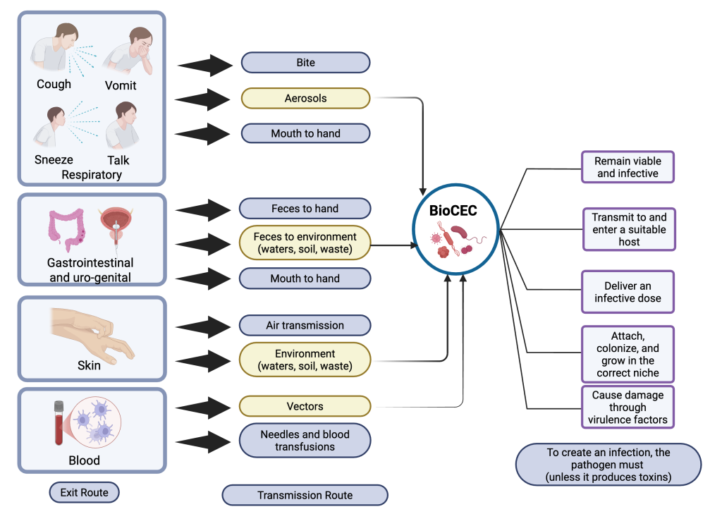
Figure 4. Exit and transmission routes for pathogens to transmit to a new host.
3.4.1 Airborne Transmission
The COVID-19 pandemic has sparked a lot of interest in respiratory infectious disease. A broad range of microorganisms (e.g., viruses, bacteria, fungal spores) from an infectious or environmental source may disperse over long distances by air currents and ultimately be inhaled or ingested. Two main factors drive airborne pathogen transmission: particle size (i.e., the diameter of the particle) and the extent of desiccation ( Cole and Cook 1998 [PPYWULGY] Cole, Eugene C., and Carl E. Cook. 1998. “Characterization of Infectious Aerosols in Health Care Facilities: An Aid to Effective Engineering Controls and Preventive Strategies.” American Journal of Infection Control 26 (4): 453–64. https://doi.org/10.1016/S0196-6553(98)70046-X. ). The particle size controls whether the particle becomes and remains airborne and infectious. Large particles fall out of the air quickly, while small particles remain airborne for a longer time. The WHO uses a particle diameter of 5 micrometers (μm) to delineate between airborne (≤5 μm) and droplet (>5 μm) transmission. Studies indicate larger particles (6 to >10 μm) deposit in the upper airway, while smaller particles penetrate deeper into the respiratory tract, or alveolar region ( Darquenne 2012 [RFYJ5FXS] Darquenne, Chantal. 2012. “Aerosol Deposition in Health and Disease.” Journal of Aerosol Medicine and Pulmonary Drug Delivery 25 (3): 140–47. https://doi.org/10.1089/jamp.2011.0916. Fernstrom and Goldblatt 2013 [XH4ZSESB] Fernstrom, Aaron, and Michael Goldblatt. 2013. “Aerobiology and Its Role in the Transmission of Infectious Diseases.” Journal of Pathogens 2013 (1): 493960. https://doi.org/10.1155/2013/493960. ). These size-based distributions are not always clear cut. Droplets settle out of air onto a surface at a velocity dictated by their mass, but in some indoor environments, air currents alter the particle’s velocity thus keeping the particle airborne.
Another critical variable is the rate at which particles desiccate. Rapid desiccation is a concern since the smaller and lighter the infectious particle, the longer it will remain airborne and the farther it will travel. Infectious agents can be expelled from the respiratory tract in a mixture of mucus and secretions, creating large, heavy particles, but rapid desiccation can lengthen the time they remain airborne as dried residuals (known as droplet nuclei, typically in the 0.5–12 μm range). Also, very large aerosol particles may initially fall out of the air only to become airborne again once they have desiccated, thus emphasizing the importance of disinfection and hygienic practices to reduce transmission ( Fernstrom and Goldblatt 2013 [XH4ZSESB] Fernstrom, Aaron, and Michael Goldblatt. 2013. “Aerobiology and Its Role in the Transmission of Infectious Diseases.” Journal of Pathogens 2013 (1): 493960. https://doi.org/10.1155/2013/493960. Fears et al. 2020 [TUR7CFWB] Fears, A. C., W. B. Klimstra, P. Duprex, et al. 2020. “Comparative Dynamic Aerosol Efficiencies of Three Emergent Coronaviruses and the Unusual Persistence of SARS-CoV-2 in Aerosol Suspensions.” Preprint, medRxiv, April 18. https://doi.org/10.1101/2020.04.13.20063784. ).
Factors such as temperature, humidity (both relative and absolute), sunlight (ultraviolet light) exposure, and even atmospheric pollutants can all act to inactivate airborne pathogens ( Tang 2009 [CWPSFBMI] Tang, Julian W. 2009. “The Effect of Environmental Parameters on the Survival of Airborne Infectious Agents.” Journal of The Royal Society Interface 6 (suppl_6): S737–46. https://doi.org/10.1098/rsif.2009.0227.focus. ). It is important to note that temperature and humidity influence viral, bacterial, and fungal particles differently. Generally, as temperature rises, virus survival decreases. Bacteria are more resistant to temperature than viruses. Temperatures above 24°C (75.2°F) typically are required to reduce airborne bacterial survival, but this is highly species dependent ( Karra and Katsivela 2007 [882UFM2X] Karra, Styliani, and Eleftheria Katsivela. 2007. “Microorganisms in Bioaerosol Emissions from Wastewater Treatment Plants during Summer at a Mediterranean Site.” Water Research 41 (6): 1355–65. https://doi.org/10.1016/j.watres.2006.12.014. ). Relative humidity is recognized as a factor in the viability of airborne and droplet viral transmissions; however, the exact relationship is currently not well understood ( Fernstrom and Goldblatt 2013 [XH4ZSESB] Fernstrom, Aaron, and Michael Goldblatt. 2013. “Aerobiology and Its Role in the Transmission of Infectious Diseases.” Journal of Pathogens 2013 (1): 493960. https://doi.org/10.1155/2013/493960. ). Fungi and their spores appear to be more resilient than viruses and bacteria, as they are often able to withstand greater stresses due to dehydration and rehydration, as well as UV radiation ( Cole and Cook 1998 [PPYWULGY] Cole, Eugene C., and Carl E. Cook. 1998. “Characterization of Infectious Aerosols in Health Care Facilities: An Aid to Effective Engineering Controls and Preventive Strategies.” American Journal of Infection Control 26 (4): 453–64. https://doi.org/10.1016/S0196-6553(98)70046-X. ).
3.4.2 Waterborne Transmission
The persistence of pathogens in water is influenced by many factors including temperature, exposure to sunlight (UV), predation, and certain chemical conditions (e.g., salinity, dissolved organic carbon), as well as settling or interactions with sediment ( Brookes et al. 2004 [UGLCRE5Z] Brookes, Justin D., Jason Antenucci, Matthew Hipsey, Michael D. Burch, Nicholas J. Ashbolt, and Christobel Ferguson. 2004. “Fate and Transport of Pathogens in Lakes and Reservoirs.” Environment International 30 (5): 741–59. https://doi.org/10.1016/j.envint.2003.11.006. ). A review by Dean and Mitchell ( Dean and Mitchell 2022 [S9LZ8KGT] Dean, Kara, and Jade Mitchell. 2022. “Identifying Water Quality and Environmental Factors That Influence Indicator and Pathogen Decay in Natural Surface Waters.” Water Research 211 (March): 118051. https://doi.org/10.1016/j.watres.2022.118051. ) cautioned that using different detection methods (i.e., culture versus molecular) may provide different results in terms of pathogen persistence. They also found that water type did not consistently affect decay, but fecal indicator bacteria decay faster in water than sediment. In addition, turbidity and temperature were found to be significantly and positively associated with indicator bacteria decay; however, sunlight and pH did not have statistically significant correlations. Overall, the effect of sunlight was more pronounced during the initial stages of decay, and over the course of time biotic interactions (i.e., predation) had a greater influence on decay than sunlight ( Dean and Mitchell 2022 [S9LZ8KGT] Dean, Kara, and Jade Mitchell. 2022. “Identifying Water Quality and Environmental Factors That Influence Indicator and Pathogen Decay in Natural Surface Waters.” Water Research 211 (March): 118051. https://doi.org/10.1016/j.watres.2022.118051. ). Generally, persistence of waterborne pathogens tends to be complicated.
4. Approaches to BioCEC Prioritization Strategies
This subsection describes different existing prioritization strategies that are widely applied to identify key variables and characterize risk from BioCEC. These strategies may inform efforts to proactively identify and develop strategies to address BioCEC. The prioritization approaches from the below examples from Health Canada, WHO, and USEPA were used in the following Tools for Prioritization to develop a guide for selecting a suitable prioritization method.
4.1 Health Canada
A QMRA is conducted to assess the potential microbiological risks associated with an infrastructure system. QMRA is a scientific approach used to estimate the risk of illness from exposure to a pathogen. Health Canada developed a QMRA model for drinking water systems and published guidance to describe their approach ( Health Canada 2018 [Q7KT2FUK] Health Canada. 2018. “Guidance on the Use of Quantitative Microbial Risk Assessment in Drinking Water.” Guidance. March 9. https://www.canada.ca/en/health-canada/programs/consultations-guidance-quantitative-microbial-risk-assessment-drinking-water/document.html. ). Although QMRA is useful as a quantitative method to assess risk and is commonly applied as a computer-based mathematical model, the QMRA perspective can be helpful in a range of applications from qualitative to quantitative. The Health Canada guidance includes general information about QMRAs, specific guidance for the Health Canada Excel-based QMRA, and a QMRA case study for a municipal water treatment plant. The following paragraphs provide more detail from the Health Canada guidance.
QMRA models assess potential risks associated with bacterial, protozoan, and viral pathogens. Assessment results are used by regulatory agencies and drinking water authorities to quantify health risks from microorganisms in water sources and develop drinking water guidelines for enteric viruses and protozoa. The approach uses the traditional hazard identification framework of exposure assessment—dose–response assessment—risk characterization. Health Canada applies QMRA across the entire drinking water system from source water to consumer.
The range from qualitative to quantitative application would start with items such as yes/no checklists (qualitative), incorporate risk matrices (semi-quantitative), and include screening assessments and probabilistic assessments with uncertainty analysis (quantitative). On the qualitative end of the spectrum, simple checklists can yield high, medium, and low risk prioritizations by tallying answers to yes/no questions. The Health Canada QMRA is especially useful at the screening assessment level for a water treatment system but is not appropriate for more advanced studies such as probabilistic assessments.
Health Canada notes that pathogen data should be considered carefully due to the small size of datasets, potential for low pathogen density, and the episodic nature of pathogen loading. For these reasons it can be difficult to characterize variability in a system. These characteristics might set BioCEC apart from other contaminants of emerging concern such as chemical contaminants. As a result, many facilities tend to rely heavily on expert judgment and literature values.
The Health Canada Excel model uses inputs such as source water pathogen concentrations, treatment system type, and ingestion/dose–response values from literature. Model results are then used to estimate the annual risk of infection and illness. The case study included in the Health Canada guidance describes a scenario wherein a municipal water treatment plant draws water from a large river that is situated in a rural, agricultural district. Decision-makers at the plant are interested in how variations in raw water quality as well as disinfection methods will affect their processes and the associated risk of infection. The case study results indicate that physical removal and disinfection processes are necessary for control of certain pathogens, and that chlorine and ozone appear to offer negligible benefits. These results offer an example of the usefulness of the Health Canada QMRA approach and can be used as a starting point for further analysis.
4.2 World Health Organization Guideline
The intended audience of the WHO report, “Quantitative microbial risk assessment: application for water safety management,” ( WHO 2016 [9LZBRAVC] WHO. 2016. “Quantitative Microbial Risk Assessment.” https://www.who.int/publications/i/item/9789241565370. ) was scientists, regulators, and water supply and sanitation system engineers and managers. The WHO report was meant to support raising awareness around how QMRA works, when it provides value for water safety management, and how it should be applied in water systems specifically. It provides detailed examples of how to use QMRA and best practices associated with the assessment based on the concept that risk assessment plays a central role in the implementation of a preventive, risk-based approach to water quality management from source to exposure for the management of microbial hazards. The document acknowledges the varying levels of expertise, data, and resources required to implement a risk-based approach. As a result, it provides several options for assessment, ranging from risk scoring in sanitary inspections and risk matrices to QMRA (Figure 5). These options need to be explored when trying to manage risk from an environmental pathogen to ensure the most suitable approach is selected.
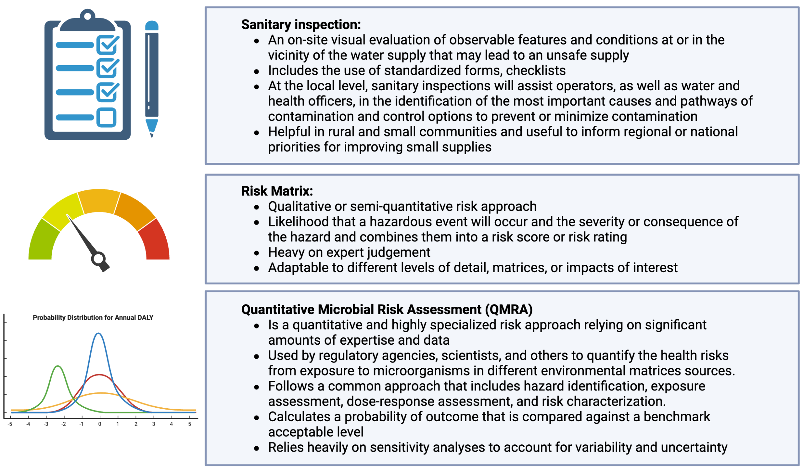
Figure 5. Risk assessment options available for risk mitigation.
4.2.1 The QMRA Framework
While exposure to infectious agents is not a new risk, all three components of the epidemiological triangle (i.e., the pathogen, host, and environment) are constantly changing, potentially impacting the risk of infection and associated risk mitigation strategies. Infectious risk statistics and indicators are for the most part measured as rates (i.e., represent an X number of individuals that have the disease per 1,000 individuals over some unit of time). This value depends on the efficacy and reliability of the disease surveillance program and has greatly underestimated the number of infections in a community.
Recognizing the deficiencies of epidemiology to characterize risk, scientists started using mathematical approaches to evaluate risk in the 1980s. These methods were further developed over the last four decades and now provide a broad range of tools to practitioners who need to perform risk assessments. QMRAs are fairly versatile and can be used to assess the potential for human risk from exposure to a known pathogen; determine critical control points in the different systems; compare specific risk mitigation, disinfection, or treatment process options to reduce the levels of various pathogens; identify and prioritize research needs; and assist in epidemiological investigations. The WHO document provides several case studies that touch on different QMRA objectives that may be of interest to the reader (see Table 2, adapted from WHO 2016 [9LZBRAVC] WHO. 2016. “Quantitative Microbial Risk Assessment.” https://www.who.int/publications/i/item/9789241565370. ).
Table 2. Summary of case studies in the World Health Organization quantitative microbial risk assessment framework
Source: Adapted from ( WHO 2016 [9LZBRAVC] WHO. 2016. “Quantitative Microbial Risk Assessment.” https://www.who.int/publications/i/item/9789241565370. ).
The WHO QMRA framework defines four specific components to all QMRAs (Figure 6): problem formulation, exposure assessment, health effects assessment, and risk characterization. This framework is similar to the traditional approach defined by others ( Haas et al. 2014 [78R697XZ] Haas, Charles N., Joan B. Rose, and Charles P. Gerba. 2014. “Quantitative Microbial Risk Assessment, 2nd Edition | Wiley.” Wiley.Com. https://www.wiley.com/en-us/Quantitative+Microbial+Risk+Assessment%2C+2nd+Edition-p-9781118910030. ), which includes hazard identification, dose–response assessment, exposure assessment, and risk characterization. Some references specifically include risk management and communication steps at the end of the QMRA process, which can be highly desirable and useful.
The problem-formulation phase defines the scope of the assessment and the overall context (i.e., the reference pathogens, exposure pathways, hazardous events, and health outcomes of interest). This would also be the stage that focuses on hazard identification. Hazard identification includes the identification of both the agent of infection and the disease outcomes. Traditionally, these outcomes range from asymptomatic infections to death, and they are highly related to pathogen virulence properties. Endemic and epidemic disease outbreak investigations, case studies, hospitalization data, and other epidemiological data sources are needed to complete this assessment. It is important to note that transmission patterns and probabilities are pathogen specific.
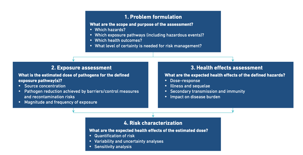
Figure 6. The World Health Organization quantitative microbial risk assessment framework.
Source: (
WHO 2016 [9LZBRAVC] WHO. 2016. “Quantitative Microbial Risk Assessment.” https://www.who.int/publications/i/item/9789241565370.
).
The objective of the exposure assessment step is to determine the frequency and magnitude of exposure to pathogens via the pathways and hazardous events defined during problem formulation. Critical quantitative information includes pathogen concentrations in environmental matrices or the fate, persistence, or decay of pathogens in barriers (e.g., treatment processes) during normal and incident situations. But other data related to exposure of humans (e.g., the size of the exposed population, vulnerability of the exposed population, frequency of exposure) are also needed.
The health effects assessment involves identifying the health impact data for the identified hazards and the specific study population. This includes the type of health effects (including secondary and/or chronic health effects that occur following initial infection), the severity and duration of illness that may occur after exposure to the pathogen, and available information on the relationship between ingested dose and the probability that health effects (infection or illness) occur (dose–response relationship). Also, the fraction and vulnerability of the population exposed may need to be considered in addition to secondary transmission and immunity. Dose–response is also a component of the health effects assessment and the mathematical relationship between the dose administered and the probability of infection or disease in the study population. The microorganisms are routinely counted in “numbers” used to count them in laboratory studies (e.g., plaque forming units, colony-forming units, (oo)cyst counts in microscopy). In dose–response experiments, traditional exposure pathways are used to measure disease and infection as endpoints. These experiments are not without limitations as culture-based assessments underestimate pathogen concentrations and molecular methods overestimate concentrations. Also, most studies use healthy individuals and less virulent pathogen strains, and few studies assess multiple combined exposure pathways.
Finally, risk characterization is the synthesis of all the information from the exposure and health effects assessments to produce a probability of occurrence and severity of adverse health effects in an exposed population. Risk characterization encompasses four distributions: (1) the spectrum of health outcomes; (2) the confidence limits around the dose–response model; (3) the distribution, occurrence, and viability of pathogens; and (4) the exposure distribution. Sensitivity analyses are recommended due to the uncertainty in the QMRA to determine the variability and uncertainty in the information at each individual step of the risk assessment and how it affects the overall risk estimate. The risk characterization is either deterministic (meaning that single values such as means are used to describe the variables used in the QMRA model) or probabilistic (meaning that statistical distributions are used to describe variables used in the QMRA model). In a deterministic QMRA, estimates of each of the QMRA model variables in the exposure and effects assessment are selected and combined to compute the resulting health risk. In a probabilistic QMRA, statistical distributions are used to describe the model variables, which reflects the stochastic (variable/uncertain) nature of most of the model variables more appropriately. The type of distribution selected considers a combination of knowledge of (pathogens in) water systems and of statistics. The health risk is computed by combining the statistical distributions using Monte Carlo methods. A wide range of software tools is available to support these calculations. Dedicated QMRA models and software tools are increasingly available to aid this risk characterization step.
Although calculated risks can be compared against a health target, users of QMRA should keep in mind that QMRA does not calculate actual disease outcomes but provides a probability that disease may occur in a specific scenario under specific circumstances. The time scale in which the risk is expressed may differ, from single-exposure events to all exposures in a year. The risk may be quantified with different endpoints, including the probability of infection, probability of illness, expected number of illness cases, and measures for burden of disease, such as disability-adjusted life years (DALYs). The need to conduct a deterministic, screening-level QMRA or a probabilistic, in-depth QMRA is primarily determined by what is needed to determine the best risk mitigation options.
The main strength of QMRA is that it is evidence-based, replicable, objective, and transparent, which allows for the discernment between risks when compared with other risk assessment approaches. Although other risk assessment approaches can also provide justification for investments in data collection and analysis improvements, QMRA can provide a more precise justification, which may be particularly useful when significant investments are required. QMRA provides a holistic system understanding; it considers all the components in the system and provides valuable information on the effects of each component on the risk of human disease associated with exposure to the pathogens. The results provide a scientific basis for evaluation of risk management priorities or control strategies. Further, QMRA enables the development of performance and specific technology targets, to determine whether or not microbial health outcome targets can be met.
4.2.2 What Does Disability-Adjusted Life Years (DALY) Mean?
Within the risk assessment literature, a number of mortality/morbidity metrics are used internationally that address human burden of diseases. These include years of life lost, quality-adjusted life years, disability-adjusted life expectancy, healthy life years, and DALYs ( Kobayashi et al. 2015 [PYBK4PDV] Kobayashi, Yumi, Greg M. Peters, Nicholas J. Ashbolt, Sean Shiels, and Stuart J. Khan. 2015. “Assessing Burden of Disease as Disability Adjusted Life Years in Life Cycle Assessment.” Science of the Total Environment 530–531 (October): 120–28. https://doi.org/10.1016/j.scitotenv.2015.05.017. ). The DALY is the metric used in WHO guidelines for the overall community health burden. The DALY is a summary measure of population health that incorporates the different severities and durations associated with different illnesses. The DALY has been applied as a metric within the WHO guidelines to provide a different relative weight to pathogens based on severity of disease outcomes. DALYs are particularly comprehensive because, in addition to the number of deaths caused, they account for years of life lost due to premature death, severity and duration of morbidity, and the number of individuals affected ( Murray and Acharya 1997 [P9Q3TTXJ] Murray, Christopher J. L., and Arnab K. Acharya. 1997. “Understanding DALYs.” Journal of Health Economics 16 (6): 703–30. https://doi.org/10.1016/S0167-6296(97)00004-0. ). It is important to include the variability (natural dispersion in a system, such as pathogen concentrations in a river) and uncertainty (lack of understanding and/or inability to measure) in all steps of the risk characterization.
One DALY represents the loss of one healthy life year. For each identified health outcome in a QMRA, DALYs are calculated as the sum of the years lost due to premature mortality and the years of productive life lost due to disability for incident cases of ill-health conditions (i.e., DALY = years of life lost + years living with a disability). Although the term disability has many meanings in different contexts, here disability refers to any short-term or long-term loss of health. To be able to calculate a DALY for each hazard or health risk, the assessor needs to identify disease outcomes to be considered (construct an outcome tree), determine the number of cases for each outcome in the population (estimate the probability associated with each outcome), identify the duration of response (years of life lost), and estimate the severity of response ( Schoen et al. 2023 [QGRLVJMP] Schoen, Mary E., Jay Garland, Jeffrey A. Soller, Sean X. Thimons, and Michael A. Jahne. 2023. “Onsite Nonpotable Water Systems Pathogen Treatment Targets: A Comparison of Infection and Disability-Adjusted Life Years (DALYs) Risk Benchmark Approaches.” Environmental Science & Technology 57 (26): 9559–66. https://doi.org/10.1021/acs.est.3c01152. ). The WHO uses a threshold of 10−6 DALYs per person per year as a benchmark to set water reuse and drinking water treatment requirements. Other organizations have used a probability of infection benchmark of 10−4 per person per year in the US for drinking water treatment requirements and for potable reuse in the State of California ( Schoen et al. 2023 [QGRLVJMP] Schoen, Mary E., Jay Garland, Jeffrey A. Soller, Sean X. Thimons, and Michael A. Jahne. 2023. “Onsite Nonpotable Water Systems Pathogen Treatment Targets: A Comparison of Infection and Disability-Adjusted Life Years (DALYs) Risk Benchmark Approaches.” Environmental Science & Technology 57 (26): 9559–66. https://doi.org/10.1021/acs.est.3c01152. ).
DALYs are subject to broad debate related to methods and efforts to quantify outcomes in economic equivalents of health interventions. For example, the capacity of individuals with some chronic disorders to adapt to their circumstances could lead to the underestimation of the health loss associated with a particular state ( Salomon et al. 2012 [3VVC2YJ8] Salomon, Joshua A., Theo Vos, Daniel R. Hogan, et al. 2012. “Common Values in Assessing Health Outcomes from Disease and Injury: Disability Weights Measurement Study for the Global Burden of Disease Study 2010.” The Lancet 380 (9859): 2129–43. https://doi.org/10.1016/S0140-6736(12)61680-8. ). In addition, the impact of disability within particular social and cultural environments can differ significantly, thus raising questions about the possibility of significant cross-cultural variability in disability weights ( Salomon et al. 2012 [3VVC2YJ8] Salomon, Joshua A., Theo Vos, Daniel R. Hogan, et al. 2012. “Common Values in Assessing Health Outcomes from Disease and Injury: Disability Weights Measurement Study for the Global Burden of Disease Study 2010.” The Lancet 380 (9859): 2129–43. https://doi.org/10.1016/S0140-6736(12)61680-8. ).
4.2.3 Best Practices in the WHO Document
The WHO ( WHO 2016 [9LZBRAVC] WHO. 2016. “Quantitative Microbial Risk Assessment.” https://www.who.int/publications/i/item/9789241565370. ) document outlines a few best practices and recommendations. For example, when relying on literature alone without site-specific data, it is often necessary to be conservative, and therefore high numbers need to be selected. In addition, relying on a sophisticated statistical analysis without holistically thinking about data inputs and assumptions would be an inadequate evaluation of system risks. Quantitatively accounting for these types of uncertainty is a challenge; however, a transparent approach to scenario analysis with point estimations provides a useful tool. Finally, in each case, these scenario calculations should be run in parallel with the “best” estimate calculations — they should not replace the best estimates. Using the upper limit of uncertainty at every stage of the model would provide a risk estimate that is unmanageably conservative and not truly representative of the population and most likely would not be very helpful for risk management. Alternatively, comparing uncertainty scenario results with the best estimates can provide useful inputs regarding model sensitivity and robustness.
4.3 US Environmental Protection Agency Contaminant Candidate List 5 for Drinking Water Supply
4.3.1 Overview
The USEPA is required by the 1996 Safe Drinking Water Act amendments (section 1412(b)(1)) to publish a list of drinking water contaminants that may cause adverse health effects in humans that are known or anticipated to occur in public water systems ( USEPA OW 2022 [QUDXR59V] USEPA OW. 2022. CCL 5 Microbial Technical Support Document. EPA 815-R-22-004. https://www.epa.gov/system/files/documents/2022-10/Technical%20Support%20Document%20for%20the%20Final%20CCL%205%20-%20Microbial%20Contaminants.pdf. ). This CCL is published approximately every five years and identifies priority contaminants for regulatory decision-making and for prioritizing research and data collection efforts. The USEPA published the first CCL for microbial contaminants, CCL 1, in 1998, and its most recent iteration, CCL 5, was published in November 2022. The CCL identifies a list of contaminants to be considered for data collection efforts and research for the Unregulated Contaminant Monitoring Rule. Contaminants are eventually considered for regulatory determination and rulemaking under the Safe Drinking Water Act only after additional data and information are collected.
The National Research Council assisted the USEPA in the development of a more robust framework for identifying and prioritizing drinking water contaminants from CCL 3 onwards. The CCL framework now consists of the following three steps (Figure 7):
- Step 1: Build a broad “universe” inclusive of all microbes that may cause human disease.
- Step 2: Screen the universe using specific exclusion criteria to generate a preliminary CCL (PCCL).
- Step 3: Score and rank the PCCL contaminants based primarily on their occurrence in drinking water and their health risk to finally yield the CCL.
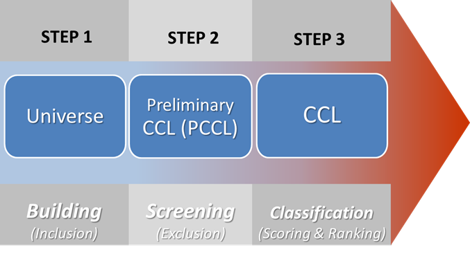
Figure 7. The Contaminant Candidate List (CCL) framework since CCL 3.
Step 1 uses a combination of literature review, input from subject matter experts, and public nominations to yield a universe of microbial contaminants capable of causing human disease. Step 2 uses 12 exclusion criteria against the contaminants in the universe to generate the PCCL. Step 3 scores the contaminants in the PCCL based on occurrence and health risk and is then ranked to give the final CCL. These steps are described in more detail in the subsections that follow.
Step 1: Building the Universe
The USEPA, upon the recommendation of the National Drinking Water Advisory Council ( NDWAC 2004 [6HR6UGCN] NDWAC. 2004. “National Drinking Water Advisory Council Report on the CCL Classification Process to the U.S. Environmental Protection Agency, May 2004.” https://www.epa.gov/sites/default/files/2014-07/documents/report_ccl_ndwac_07-06-04.pdf. ), began to specifically use Taylor et al. ( Taylor et al. 2001 [BD5A7NUS] Taylor, L. H., S. M. Latham, and M. E. Woolhouse. 2001. “Risk Factors for Human Disease Emergence.” Philosophical Transactions of the Royal Society B: Biological Sciences 356 (1411): 983–89. https://doi.org/10.1098/rstb.2001.0888. ), a comprehensive literature review identifying species of infectious organisms known to be pathogenic to humans, and more recent literature reviews as the starting point for building the microbial universe for CCL 3. This resulted in a total of 1,425 microbes in the universe for CCL 3: 1,415 from Taylor et al. ( Taylor et al. 2001 [BD5A7NUS] Taylor, L. H., S. M. Latham, and M. E. Woolhouse. 2001. “Risk Factors for Human Disease Emergence.” Philosophical Transactions of the Royal Society B: Biological Sciences 356 (1411): 983–89. https://doi.org/10.1098/rstb.2001.0888. ), and 10 from additional literature reviews. These 1,425 pathogens have been carried forward in the subsequent CCL 4 and CCL 5, with the added step of seeking feedback from subject matter experts. Starting with CCL 5, a new phase of seeking public nominations (Figure 8) was introduced to the universe building stage. The public nominations committee asked for the name of the pathogen and for data evidence, such as the pathogen’s likely occurrence in public water systems and its health effects, that would make it potentially require regulation. The public nomination phase yielded 16 unique microbial contaminants for consideration for CCL 5. CCL 5 generated a universe consisting of 1,435 microbes after minor changes to nomenclature and consolidation of some members.
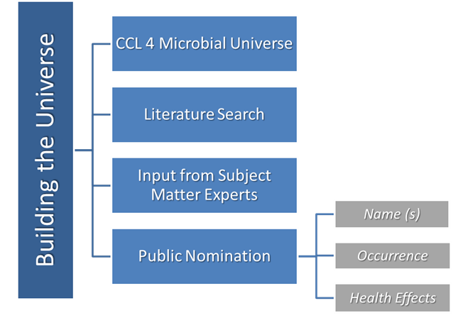
Figure 8. Step 1 of the Contaminant Candidate List 5 framework: building the universe.
Source: Adapted from (
USEPA OW 2022 [QUDXR59V] USEPA OW. 2022. CCL 5 Microbial Technical Support Document. EPA 815-R-22-004. https://www.epa.gov/system/files/documents/2022-10/Technical%20Support%20Document%20for%20the%20Final%20CCL%205%20-%20Microbial%20Contaminants.pdf.
).
Step 2: Screening
For the screening step, 12 exclusion criteria were developed to screen the microbial universe developed in Step 1. The exclusion criteria focused on plausibility of pathogen presence, survival, and transport through drinking water to disease manifestations from drinking water exposure ( USEPA OW 2022 [QUDXR59V] USEPA OW. 2022. CCL 5 Microbial Technical Support Document. EPA 815-R-22-004. https://www.epa.gov/system/files/documents/2022-10/Technical%20Support%20Document%20for%20the%20Final%20CCL%205%20-%20Microbial%20Contaminants.pdf. ). The specific exclusion criteria were as follows:
- Anaerobes (microorganisms that cannot survive in oxygenated environments)
- Fastidious or obligate intracellular pathogens (environmental survival in water implausible)
- Pathogens exclusively transmitted by direct or indirect contact with blood or body fluids (including sexually transmitted diseases)
- Pathogens transmitted by vectors
- Microflora common to the gastrointestinal tract, skin, and mucous membranes
- Pathogens transmitted solely by respiratory secretions
- Pathogens whose life cycle is incompatible with drinking water transmission
- Pathogens where drinking water–related transmission is not implicated
- Natural habitat is in the environment without epidemiological evidence of drinking water–related disease and without evidence of drinking water–related nosocomial (i.e., hospital-based) infection
- Pathogens not endemic to North America
- A genus and species or serotype may be chosen to represent a group of closely related organisms
- Current taxonomy does not support the classification listed by Taylor et al. ( Taylor et al. 2001 [BD5A7NUS] Taylor, L. H., S. M. Latham, and M. E. Woolhouse. 2001. “Risk Factors for Human Disease Emergence.” Philosophical Transactions of the Royal Society B: Biological Sciences 356 (1411): 983–89. https://doi.org/10.1098/rstb.2001.0888. )
The screening step eliminated 1,400 of the 1,435 pathogens, leaving only 35 pathogens on the PCCL (Table 3).
Table 3. Pathogens screened from the universe using exclusion criteria
| Pathogen Class | Total (Universe) | Pathogens Excluded | PCCL |
| Bacteria | 545 | 527 | 18 |
| Viruses | 225 | 218 | 7 |
| Protozoa | 66 | 59 | 7 |
| Helminths | 286 | 286 | 0 |
| Fungi | 313 | 310 | 3 |
| Total | 1,435 | 1,400 | 35 |
Note: PCCL is preliminary contaminant candidate list
Source: Adapted from ( USEPA OW 2022 [QUDXR59V] USEPA OW. 2022. CCL 5 Microbial Technical Support Document. EPA 815-R-22-004. https://www.epa.gov/system/files/documents/2022-10/Technical%20Support%20Document%20for%20the%20Final%20CCL%205%20-%20Microbial%20Contaminants.pdf. ).
Step 3: Classification
The classification step takes the PCCL generated in the screening step and puts each pathogen on that list through a scoring system focusing on two categories: (1) its occurrence in public water systems and (2) its health risk for causing adverse health effects in humans. The occurrence scoring relies on a combination of waterborne disease outbreak (WBDO) data from the CDC’s Morbidity and Mortality Weekly Reports ( Benedict et al. 2017 [GI2JCKTQ] Benedict, Katharine M., Hannah Reses, Marissa Vigar, et al. 2017. “Surveillance for Waterborne Disease Outbreaks Associated with Drinking Water — United States, 2013–2014.” MMWR. Morbidity and Mortality Weekly Report 66 (44): 1216–21. https://doi.org/10.15585/mmwr.mm6644a3. ) or pathogen occurrence data in drinking water and source water. The higher of the two scores (either WBDO or occurrence in drinking/source water) is selected for the occurrence criteria. The WBDO scoring follows a five-level hierarchy (i.e., scores ranging from 5 to 1) using the following classifications:
- 5: Has caused two or more WBDOs in the US as reported by the CDC between 2009 and 2017.
- 4: Has caused at least one WBDO in the US as reported by the CDC between 2009 and 2017.
- 3: Has caused documented WBDOs any time in the US.
- 2: Has caused documented WBDOs in countries other than the US.
- 1: Has never caused WBDOs in any country but has been epidemiologically associated with water-related disease.
Pathogen occurrence in drinking/source water scoring follows a three-level hierarchy:
- 3: Detected in drinking water in the US.
- 2: Detected in source water in the US.
- 1: Not detected in the US.
From the range of hierarchies listed above, it is obvious that WBDO data can result in a higher score for the first term in Equation 1 than simply the occurrence data for the pathogen in drinking/source water.

Equation 1.
The health risk scoring follows a 7-level scoring hierarchy for the general population, as well as four sensitive subpopulations: children/infants, the elderly, pregnant women, and people with chronic disease. The highest score of 7 is given when there is significant mortality involved (>1/1,000 cases) while the lowest score of 1 is reserved for mild symptoms with minimal or no impact on daily activities. The summative score for the health risk for the two populations (i.e., second term of Equation 1) is then normalized by a correction factor representing the five types of populations divided by 2× the score range for the two populations.
All 35 pathogens on the PCCL were scored using the criteria described above, and then a total score was calculated for each using Equation 1. After sorting the 35 pathogens from highest to lowest total score, the top 12 pathogens were selected as the final pathogens for CCL 5 (Table 4).
Table 4. Final Contaminant Candidate List 5 consisting of the 12 highest-ranked pathogens
| Pathogen | Ranking | WBDO | Occurrence | Health | Total Score |
| Naegleria fowleri | 1 | 5 | 3 | 5.0 | 10.0 |
| Legionella pneumophila | 2 | 5 | 3 | 3.6 | 8.6 |
| Escherichia coli (O157) | 3 | 5 | 3 | 3.2 | 8.2 |
| Pseudomonas aeruginosa | 4 | 5 | 3 | 3.2 | 8.2 |
| Helicobacter pylori | 5 | 1 | 3 | 5.0 | 8.0 |
| Campylobacter jejuni | 6 | 5 | 3 | 2.5 | 7.5 |
| Mycobacterium abscessus | 7 | 4 | 3 | 3.2 | 7.2 |
| Shigella sonnei | 8 | 4 | 3 | 3.2 | 7.2 |
| Caliciviruses | 9 | 5 | 3 | 2.1 | 7.1 |
| Mycobacterium avium | 10 | 4 | 3 | 2.9 | 6.9 |
| Adenovirus | 11 | 2 | 3 | 3.6 | 6.6 |
| Enterovirus | 12 | 2 | 3 | 3.6 | 6.6 |
Note: WBDO is waterborne disease outbreak.
Source: Adapted from ( USEPA OW 2022 [QUDXR59V] USEPA OW. 2022. CCL 5 Microbial Technical Support Document. EPA 815-R-22-004. https://www.epa.gov/system/files/documents/2022-10/Technical%20Support%20Document%20for%20the%20Final%20CCL%205%20-%20Microbial%20Contaminants.pdf. ).
4.3.2 Limitations
A number of limitations exist in the CCL 5 prioritization framework. Specifically, exclusion criteria 1, 9, and 10 have been previously challenged by the CCL 4 Science Advisory Board. For example, exclusion criterion 1 was challenged because of the presence of spore-forming anaerobes that survive oxygenated environments. For exclusion criterion 9, nosocomial infections were included in the criterion from CCL 4 to CCL 5, and concern for the presence of pathogens in distribution systems was recognized owing to factors such as biofilms. Criterion 10 remained unchanged after further review by the USEPA. Lastly, the WBDO disease outbreak data from the CDC is largely believed to be underreported for multiple reasons, including the variability in surveillance capabilities across states.
5. Tools for Prioritization
Several tools can be used to understand the risk associated with BioCEC including surveys, a risk matrix, or QMRA ( WHO 2016 [9LZBRAVC] WHO. 2016. “Quantitative Microbial Risk Assessment.” https://www.who.int/publications/i/item/9789241565370. ). The selection of a tool to use depends on the expertise of the individuals conducting the risk assessment, their experience with advanced statistical assessment, and the availability of data. For some BioCEC, the limited availability of data necessitates the use of a qualitative or semi-quantitative approach; however, the use of qualitative and semi-quantitative approaches is still powerful. A guide to selecting the type of approach to apply is shown below in a flowchart (Figure 9).
Surveys for evaluating BioCEC, for example, sanitary surveys, may be generated in-house or by a national or international organization. Although sanitary surveys are traditionally used in water supply systems in the US, a sanitary survey can also be used as a more holistic method to investigate the sources of fecal contamination to a waterbody. Sanitary surveys can be used for drinking water, shellfish, and watershed protection programs, as well as beaches and other recreational waters. Surveys or checklists can be developed to qualitatively compare risks associated with different BioCEC at a specific site. It allows operators or inspectors to provide a binary answer to questions about the presence of specific BioCEC (yes or no) and to broadly classify the risk associated with each (from very high risk to low risk). Surveys can also be used in conjunction with environmental parameters (e.g., water quality data) to provide additional means of prioritization based on data. The strength of a survey or checklist is that it is straightforward and requires the fewest resources to complete, which also means that it may be feasible to update more frequently. A limitation of the survey approach is that it may not capture all potential hazards.
The next step up in complexity and knowledge required is a risk matrix, which can be either qualitative or semi-quantitative ( WHO and International Water Association 2009 [N3SWAM7S] WHO, and International Water Association. 2009. Water safety plan manual: step-by-step risk management for drinking-water suppliers. World Health Organization. https://iris.who.int/handle/10665/75141. Fewtrell and Bartram 2001 [5L94W9KQ] Fewtrell, Lorna, and Jamie Bartram, eds. 2001. Water Quality: Guidelines, Standards, and Health: Assessment of Risk and Risk Management for Water-Related Infectious Disease. World Health Organization Water Series. World Health Organization. ). In the qualitative approach, experts can classify the risk from a given BioCEC based on its severity or consequence and the likelihood or frequency. In the semi-quantitative approach, different BioCEC are given scores that can then be totaled and ranked. This semi-quantitative approach was used by the USEPA to rank the list of BioCEC to generate the Microbial CCL5 ( USEPA OW 2022 [QUDXR59V] USEPA OW. 2022. CCL 5 Microbial Technical Support Document. EPA 815-R-22-004. https://www.epa.gov/system/files/documents/2022-10/Technical%20Support%20Document%20for%20the%20Final%20CCL%205%20-%20Microbial%20Contaminants.pdf. ).
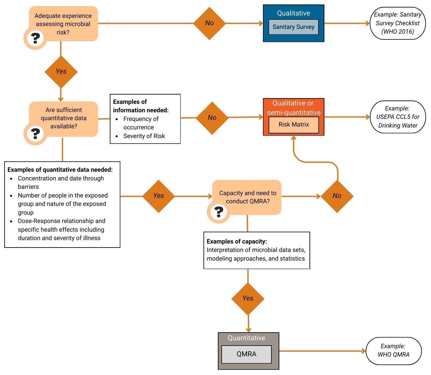
Figure 9. Approaches applied to assess the risk of biological contaminants of emerging concern.
The advantage of a risk matrix is that it can capture different types of risks and tends to cover a wider range of events relative to a survey or checklist. It can be challenging to be consistent in the application of risk scores for different types of hazards and to determine the likelihood of different events.
QMRA is a systematic approach to decision-making and prioritization of risks. Examples of the types of data required for completing a QMRA include understanding the BioCEC occurrence, variability, and fate through different barriers. The analysis also includes the number of people exposed to the pathogen, the various routes of exposure, and the type of people in the exposed group, such as the elderly or children. In addition, the dose–response relationship and specific health effects, including duration and severity of the illness, are needed to complete a QMRA. Relative to a survey or risk matrix, the QMRA provides the most systematic and rigorous approach to the comparison of different risks; however, the QMRA requires significant data, statistical knowledge, and expertise.
6. Limitations and Knowledge Gap
The Interstate Technology and Regulatory Council’s BioCEC team conducted a nationwide survey with the goal of understanding current practices in different states. One of the questions asked during this survey was how states and agencies approach the prioritizing and monitoring of BioCEC. The responses indicated that there are significant variations between the responders with the majority relying on federal guidance and requirements. Most states and agencies do not have a prioritized list of BioCEC, while some states, such as Alabama and New Hampshire, have partial prioritization schemes (that focus on specific contaminants), such as harmful algal blooms and Legionella. When prioritization occurs, it is influenced by factors such as federal guidance, resource availability, risk to public health, and federal requirements. In terms of monitoring, a majority of the states are not monitoring for unregulated BioCEC, while some states such as Vermont are monitoring for specific unregulated BioCEC related to site-specific events, such as cyanobacterial blooms. In Utah, spot monitoring is conducted for unregulated BioCEC when there is a reason for concern, such as reported outbreaks. Common triggers for starting monitoring programs were identified as federal requirements, known or suspected releases, public health concerns, and availability of funding. Although monitoring programs and collecting data are key to evaluating BioCEC, the primary limitations for widespread monitoring programs are available resources and funding.
Different prioritization schemes were presented in this guidance, including WHO’s guideline and USEPA’s CCL5 list. Although these resources provide generalized best practices and recommendations to use qualitative and quantitative data or information to prioritize BioCEC, evaluation of specific risk may be highly site and scenario specific. This requires significant expertise and resources when developing a strategy or approach to evaluate risk. In addition, criteria developed to define a prioritization approach, such as exclusion basis, could be debatable, and it may be difficult to have full agreement among subject experts, as presented in US Environmental Protection Agency Contaminant Candidate List 5 for Drinking Water Supply on CCL5. Some of the tools used to evaluate risk, such as QMRA, require significant data and information, such as established dose–response models and occurrence data. Particularly with emerging BioCEC, this information may not be readily available in the literature and may require research and significant resources to conduct monitoring campaigns and establish dose–response models. In those cases, to make timely decisions to protect public health, relevant surrogate pathogen data can be used to estimate persistence, dose–response, or other variables until BioCEC data become available. For example, the Water Environment Federation COVID-19 guidance for water and wastewater systems relied on surrogate viruses to estimate risk ( Water Environment Federation 2020 [ZX4BIT9D] Water Environment Federation. 2020. “The Water Professional’s Guide to COVID-19.” https://www.wef.org/the-water-professionals-guide-to-the-2019-novel-coronavirus. ). In the use of QMRA to evaluate water reuse, the USEPA identified data on pathogen densities in source water, viral load estimation methods that inform viability and infectivity, lack of dose–response data for enteric viruses, and understanding health burden ( Jahne et al. 2025 [33MUS2YQ] Jahne, M., S. Nappier, J. Garland, M. Schoen, and J. Soller. 2025. “Risk-Based Framework for Developing Microbial Treatment Targets for Water Reuse.” U.S. Environmental Protection Agency. https://cfpub.epa.gov/si/si_public_record_Report.cfm?dirEntryId=363921&Lab=CESER. ) associated with reference pathogens as some of the critical knowledge gaps. Overall, the number of key variables that correspond to a high-risk BioCEC are vast, complex, and highly interlinked, which makes prioritization of BioCEC a highly involved and multi-step process as presented in Approaches to BioCEC Prioritization Strategies.